An Inconvenient Probability v5.13
Source: An Inconvenient Probability v5.13
Publisher: Michael’s Substack (Free) | Author: Michael’s Substack (Free)
Published: March 14, 2024 | Archived: July 13, 2026
\[This version is substantially changed from V4 by using more relevant priors better integrated with the basic observations for simplicity. The lack of independence between when/where/what features under the lab leak hypothesis is now made explicit from the start rather than patched in. Just as I was about to post, new data on planned sequence features became available, so this update coincidentally includes not only some change in form but also an appreciable change in the odds. 5.11 dropped a factor that was based on my misreading of a paper. 5.12 uses an improved method of allowing for sequences in related viruses. Some of the introductory remarks are anachronistic, but I’ve written about the current politics [elsewhere](https://michaelweissman.substack.com/p/trump-on-covid-lab-leak). ***The method remains explicitly ready for correction based on improved reasoning or new evidence.*** \[Last notable revision 5.11→5.12 11/10/2025\]
Early on in the Covid pandemic, I took a preliminary look at the relative probabilities that SARS-CoV-2 (SC2) came from some sort of lab leak vs. more traditional direct zoonotic paths. Although zoonotic origins have been more common historically, the start in Wuhan where the suspect lab work was concentrated left the two possibilities with comparable probabilities. That result seemed convenient because it left strong motivation both to increase surveillance against future zoonosis and to stringently regulate dangerous lab work. Since then there have been major changes in circumstances that change both the balance of the evidence and the balance of the consequences of looking at the evidence. I think these warrant taking another look.
The origins discourse has become increasingly polarized with different opinions often tied to a package of other views. To avoid having some readers turn away out of aversion to some views that have become associated with the suspicion of a lab leak, it may help to first clarify why I think the question is important and to name some of the claims that I’m not making before plunging into the more specific analysis of probabilities.
I’m now more concerned about dangerous work being accelerated rather than useful work being over-regulated. This is not a specifically Chinese problem. Work with dangerous new viruses has been done, is underway, or is planned in Madison, the Netherlands, Australia, and South Korea, with some questionable work in Boston. I’m not suggesting that the US or other western governments should officially say that they think SC2 started from a Wuhan lab. That would make it harder to work with China on the crucial issues of global warming and even on international pathogen safety regulation itself. (I just signed a letter “urging renewal of US-China Protocol on Scientific and Technological Cooperation”.) I’m definitely not endorsing the cruel opposition to strenuous public health measures that seems to have become associated with skepticism about the zoonotic account.
In what follows I will try to objectively calculate the odds that SC2 came from a lab, in the hope that will be useful to anyone thinking about future research policy. The underlying motivation for this effort has been eloquently described by David Relman, who has also provided a nice non-quantitative outline of the general types of evidence supporting different SC2 origins hypotheses.
Looking forward, what we really care about is estimating risks. We already know from experience that the risks of zoonotic pandemics are significant. Are the risks of some types of lab work comparably significant? We shall use some prior estimates of those risks on the way to answering a more concrete question– does it look like SC2 came from a lab? If the answer is “probably not”, then it’s at least possible that the prior estimates of significant lab risk may have been overstated, although the evidence for that would be skimpy. If the answer is “probably yes” that indicates that the prior estimates of significant risk should not have been ignored.
The method used may also help readers to evaluate other important issues without relying too much on group loyalties. The method is explicitly ready for correction based on improved reasoning or new evidence.** Our method will be robust Bayesian analysis, a systematic way of updating beliefs without putting too much weight on either one’s prior beliefs or the new evidence. Bayesian analysis does not insist that any single piece of evidence be “dispositive” or fit into any rigid qualitative verbal category. Some hypotheses can start with a big subjective head-start, but none are granted categorical qualitative superiority as “null hypotheses” and none have to carry a qualitatively distinct “burden of proof”. Each piece of evidence gets some quantitative weight based on its consistency with competing hypotheses. The consistency with evidence then allows us to substantially change our prior guesses so that the final probability estimate is not just a recycling of our initial opinions.
In practice there are subjective judgments not only about the prior probabilities of different hypotheses but also about the proper weights to place on different pieces of evidence. I will use hierarchical Bayes techniques to take into account the uncertainty in the impacts of different pieces of evidence and “Robust Bayesian analysis” to allow for the uncertainty in the priors.
There have been about a dozen more-or-less-published Bayesian analyses of SC2 origins, other than my own very preliminary inconclusive one. The ones that attempt to be comprehensive and were published before the first version of this blog all came to conclusions similar to the one I shall reach here. Starting in early 2024 several have come out favoring a zoonotic spillover at a market. All are discussed in Appendix 1.
I will focus on comparing the probability that SC2 originated in wildlife vs. the probability that it originated in work similar to that described in the 2018 DEFUSE grant proposal submitted to the US Defense Advanced Research Project Agency from institutions that included the University of North Carolina (UNC), the Duke National University of Singapore, and the EcoHealth Alliance (EHA) as well as the Wuhan Institute of Virology (WIV). (For brevity I’ll just refer to this proposal as DEFUSE.) Although DEFUSE was not funded by DARPA, anyone who has run a grant-supported research lab knows that work on yet-to-be-funded projects routinely continues except when it requires major new expenses such as purchasing large equipment items. Some closely related work was described shortly later in an NIH grant application from EHA and WIV and in a grant to WIV from the Chinese Academy of Sciences. When Der Spiegel asked Shi Zhengli, the lead coronavirus researcher at WIV, whether the work had started anyway she responded “I don’t want to answer this question…”
I will not discuss any claims about bioweapons research. It is not exactly likely that a secret military project would request funding from DARPA for work shared between UNC and WIV.
My analysis will not make use of the rumors of roadblocks around WIV, cell-phone use gaps, sick WIV researchers, disappearances of researchers, etc. That sort of evidence might someday be important but at this point I can’t sort it out from the haze of politically motivated reports. Mumbled inconclusive evidence-free executive summaries from various agencies are even less useful. I will discuss in passing two recent U.S. government funding decisions that could potentially provide weak evidence concerning the actual probabilities as seen by those with inside information. The biological and geographic data are much more suited to reliable analysis.
The main technical portions will be unpleasantly long-winded since for a highly contentious question it’s necessary to supply supporting arguments. Although parts may look abstract to non-mathematical readers, all the arguments will be accessible and transparent, in contrast to the opaque complex modeling used in some well-known papers. For the key scientific points I will provide standard references. At some points I bolster some arguments with vivid quotes from key advocates of the zoonotic hypothesis, providing convenient links to secondary sources. The quotes may also be obtained from searchable .pdf’s of slack and email correspondence.
The outline is to
1. Give a short non-technical preview.
2. Introduce the robust Bayesian method of estimating probabilities, along with some notation.
3. Discuss a reasonable rough consensus starting point for the estimation, i.e. the prior odds for a pandemic of this sort starting in Wuhan in 2019 via routine processes unrelated to research or via research-related activities.
4. Discuss whether the main papers that have claimed to demonstrate a zoonotic origin via the wildlife trade should lead us to update our odds estimate.
5. Update the odds estimate using a variety of other evidence, especially sequence features.
6. Present brief thoughts about implications for future actions.
I will denote three general competitive hypotheses:
ZW: zoonotic source transmitted via wildlife to people, suspected via a wet-market.
ZL: zoonotic source transmitted to people via lab activities sampling, transporting or otherwise handling viruses.
LL: a laboratory-modified source, leaked in some lab mishap.
At points I’ll divide the ZW hypothesis into two branches ZWM involving a spillover from an intermediate host at the Huanan Seafood Market (HSM) and all other ZW’s, ZWO. This division is useful because there has been a substantial amount of evidence cited (tending both for and against) that is pertinent only to the ZWM sub-hypothesis.
The viral signatures of ZW and ZL would be similar, so the ratio of their probabilities would be estimated from knowledge of intermediate wildlife hosts, of the lab practices in handling viral samples, and detailed locations of initial cases. Demaneuf and De Maistre wrote up a careful Bayesian discussion of that issue in 2020, before the DEFUSE proposal for modifying coronaviruses was publicly known. They concluded that the probability of ZW, i.e. P(ZW), and the probability of ZL, i.e. P(ZL), were about equal.
Much of their analysis, particularly of prior probabilities, is close to the arguments I use here, but written more gracefully and with more thorough documentation. They use a different way of accounting for uncertainties than I do, but unlike some other estimates their method is transparent and rational. Here I’ll focus on comparing the probability P(ZW) to that of the LL lab account, P(LL), because sequence data point to a lab involvement in generating the viral sequence, so that P(ZL) will itself be somewhat smaller than P(LL). (I’ve added Appendix 5 to discuss the ZL probability.)
Ratios of probabilities such as P(LL)/P(ZW) are called odds. It’s easier to think in terms of odds for most of the argument because the rule for updating odds to take into account new evidence is a bit simpler than the rule for updating probabilities.
I’ll start with odds that heavily favor ZW since historically most new epidemics do not come from research activities. Then I’ll update using several important facts. The most basic what/where/when facts are that SC2 is a sarbecovirus that started a pandemic in Wuhan in 2019. Wuhan is the location of a major research lab that had not long before the outbreak submitted the DEFUSE grant proposal that included plans to collect bat sarbecoviruses and modify them in ways later found in SC2. That location, timing, and category of virus could also have occurred by accidental coincidences for ZW, but we shall see that it’s not hard to approximately convert the coincidences to factors objectively increasing the odds of LL. Here’s a beginning non-technical explanation of how the odds get updated.
I’ll start with a consensus view, that the prior guess would be that overall P(LL) is much less than P(ZW). That corresponds to the standard idea that you would call ZW the null hypothesis, i.e. the boring first guess. Rather than treat the null as qualitatively sacred I’ll just leave it as initially quantitatively more probable by a crudely estimated factor.
Now we get to the simple part that has often been either dismissed or over-emphasized. Both P(ZW) and P(LL) come from sums of tiny probabilities for each individual person. P(LL) comes mostly from a sum over individuals in Wuhan. P(ZW) comes from a sum over a much larger set of individuals spread over China and southeast Asia. Since we know with confidence that this pandemic started in Wuhan, restricting the sum of individual probabilities to people around Wuhan doesn’t reduce the chances for LL much but eliminates most of the contributions to the chances for ZW. Wuhan has less than 1% of China’s population, so ~99% of the paths to ZW are crossed off. That means we need to increase whatever P(LL)/P(ZW) odds we started with by about a factor of 100.
Further updates following the same logic come from other data. A natural outbreak could come from any of a diverse collection of pathogens, but this outbreak matched the specific subcategory of virus being studied in the Wuhan labs. Another update will come from a special genetic sequence that codes for the furin cleavage site (FCS) where the UNC-WIV-EHA DEFUSE proposal suggested adding a tiny piece of protein sequence to a natural coronavirus sequence. The tiny extra part of SC2’s spike protein, the FCS that is absent in its wild relatives, has nucleotide coding that is rare for related natural viruses but seems less peculiar for the most relevant known designed sequences, the mRNA vaccines. A similar update involves a pattern of how the virus sequence can be cut into pieces by some lab restriction enzymes, a pattern closely matching plans in DEFUSE drafts but quite rare in natural viruses. We can again make approximate numerical estimates of how much more coincidental such features seem for a natural origin than for a lab origin.
Even if we start with a generously high but plausible preference for ZW, once the evidence-based updates are done we’ll have P(LL) much larger than P(ZW). P(ZW) will shrink to less than 1%, and is saved from shrinking much further only by allowance for uncertainties.
An analogy may help clarify the method for those who have never used it before. Say that you’ve been hanging out in your house for a few hours. At some point you turn on a light in the kitchen. A few minutes after that you smell burning electrical insulation in the kitchen. Even though fires are not usually caused by faulty electrical wiring in kitchens, you would rightly suspect that this one was. Bayesian reasoning allows you to systematically express and evaluate the intuitions behind that suspicion.
This openly crude and approximate form of argument may alarm readers who are not accustomed to the Fermi-style calculations routinely used by physicists. In this sort of calculation one doesn’t worry much about minor distinctions between similar factors, e.g. 8 and 12, because the arguments are not generally that precise. Sometimes the large uncertainties in such a calculation render the conclusion useless, but this turns out not to be one of those cases.
The standard logical procedure to calculate the odds, P(LL)/P(ZW), is to combine some rough prior sense of the odds with judgments of how consistent new pieces of evidence are with the LL and ZW hypotheses. Bayes’ Theorem provides the rule for how to do this. (See e.g. this introduction.)
One starts with some roughly estimated odds based on prior knowledge:
P0(LL)/P0(ZW). Then one updates the odds based on new observations. The conditional probabilities that you would see those observations if a hypothesis (either LL or ZW) were true are denoted P(observations|LL) and P(observations|ZW), called the “likelihoods” of LL and ZW. Each conditional probability is evaluated without regard to whether the hypothesis itself is probable or not.
Rather than categorizing each unusual feature as either a smoking gun or mere coincidence, Bayesian analysis assigns each feature a quantitative odds update factor. Events that are unusual under some hypothesis do not rule out that hypothesis but they do constitute evidence against it if the events are more likely under a competing hypothesis. Our task here is to try to turn each qualitative surprise into a rough quantitative likelihood ratio.
Assuming these likelihoods are themselves known, Bayes’ Theorem tells us the new “posterior” odds are
P(LL)/P(ZW) = (P0(LL)/P0(ZW))*(P(observations|LL)/P(observations|ZW)).
In practice, it’s hard to reason about all the observations lumped together, so we break them up into more or less independent pieces, to the extent that can be done, and do the odds update using the product of the likelihood ratios for those pieces.
P(LL)/P(ZW) =
(P0(LL)/P0(ZW))(P(obs1|LL)/P(obs1|ZW))(P(obs2|LL)/P(obs2|ZW))…… *(P(obsn|LL)/P(obsn|ZW))
At several key points we’ll see that several aspects of the observations would not be close to independent under one or the other of the hypotheses, so we’ll be careful in those cases not to break up the likelihoods into separate factors.
At this point it’s necessary to recognize that not only the prior odds
P0(LL)/P0(ZW) but also the likelihoods involve some subjective estimates. In order to obtain a convincing answer we need to include some range of plausible values for each likelihood ratio. As we shall see, inclusion of the uncertainties is important because realistic recognition of the uncertainties will tend to pull the final odds back from an extreme value towards one.
Once our odds become products of factors of which more than one have some range of possible values, our expected value for the product is no longer equal to the product of the expected values. Since the expected value of a sum is just the sum of the expected values it’s convenient to convert the product to a sum by taking the logarithms of all the factors.
ln(P(LL)/P(ZW)) = ln(P0(LL)/P0(ZW))+ln(P(obs1|LL)/P(obs1|ZW)) … +ln(P(obsn|LL)/P(obsn|ZW)) = logit0 + logit1 … +logitn
where “logit” is used for brevity. The logarithmic form has the added advantage that the typical error bars around the best estimate are often about symmetrical.
At each stage I will include a crude estimate of the log of each likelihood and of its uncertainty expressed as a standard error of that log. Standard hierarchical Bayes techniques then down-weight factors with big uncertainty. The resulting down-weighted logits for factors with big uncertainty (si) tend to be smaller than the initial crude estimates of the logs of the likelihood ratios(Li) The technique used is described in Appendix 3. The results are not sensitive to the details because I do not use likelihood ratios with large si. The down-weighted results are the logits used.
Once the net likelihood factor is estimated, taking uncertainties into account, we still have a distribution of plausible prior odds. This can also be treated by assuming
a probability distribution around the point estimate of the log odds. The final odds will be obtained from integrating the net probabilities, including the net likelihood factor, over that distribution. This distribution is wide enough to make its form, not just its standard deviation, potentially important for the result.
The treatments of the priors and the likelihoods look superficially similar, but are not equivalent. Uncertainty in the likelihoods leads to discounting the likelihood ratios but not to discounting the priors. Uncertainty in the priors leads to discounting both. Thus observations with uncertain implications leave the priors untouched but highly uncertain priors can make fairly large likelihood ratios irrelevant. Since in this case the priors tend toward ZW but the likelihoods tend more strongly toward LL the inclusion of each type of uncertainty will substantially reduce the net odds favoring LL.
Often our hypotheses can be broken up into sub-hypotheses. For example, ZW can occur via market animals or directly from a bat, among other possibilities. LL can occur at WIV or at the Chinese CDC. There’s nothing wrong or contradictory in summing probabilities over sub-hypotheses. In calculating these contributions, however, it is crucial to separately multiply the chain of observational factors for each contributing sub-hypothesis and then add the resulting probabilities rather than adding the probabilities at each observational step and then multiplying. For example, if a hypothesis is that some cookies were stolen by a team of animals consisting of a snake and a pig knowing that that team can get through a small opening and can knock down a wall does not give any probability that they stole a cookie which could only be reached by getting through a small hole and then knocking down a wall. Neither sub-hypothesis (snake or pig) works although a coarse grained look would say that the snake/pig team has good chances of both hole-threading and wall-smashing. This issue will come up several times in important if less extreme contexts.
Along the way we shall see several observed features that perhaps should give important likelihood factors that I think tend to favor LL but for which there’s substantial uncertainty and thus little net effect. I will just drop these to avoid cluttering the argument with unimportant factors. I will include some small factors when the sign of their logit is unambiguous, e.g. a factor from the lack of any detection of a wildlife host. I will not omit any factors that I think would favor ZW. I’ll take care not to penalize ZW’s odds for features that might seem peculiar under the ZW hypothesis but that would seem needed for a zoonotic virus to be able to cause a notable pandemic.
My analysis differs from some others in one important respect. The others treat “DEFUSE” as an observation and try to estimate something like P(DEFUSE|LL)/P(DEFUSE|ZW). I don’t see how to do that. Instead I treat DEFUSE (along with the closely related follow-up grants) as a way to define a particular branch of the LL hypothesis. Since it’s narrower than generic LL, it should be easier to find observations that don’t fit it, i.e. have low likelihoods. The flip side of that is that observed features that it does fit give higher likelihoods than they would for generic LL. Picking a reasonable prior for a leak of something stemming from DEFUSE-style work given the existence of the proposal will require looking more at prior estimates of lab leak probabilities rather than at the sparse history of previous pandemics. In earlier versions I used those estimates as a sanity check on more broadly inferred priors but here I switch those roles.
We will use priors based on attempts to predict yearly rates of spillovers from ongoing lab work based on prior knowledge of lab events. To the extent that those estimates are already reliable our whole exercise here is only of historical interest, since those estimates tell us directly to take lab risks seriously regardless of the source of this particular pandemic. Our priors, however, are far from precise, so looking at the evidence for this one pandemic will help us refine them. For practical purposes, we are only interested in estimating the source of this one pandemic in order to check the credibility of the warnings.
Let’s start with the fuzzy generic prior odds just to get a rough feel of what’s plausible. In my lifetime, starting in 1949, there have been seven other significant (>10k dead) worldwide pandemics. At least one pandemic (1977 A/H1N1) came from some accident in dealing with viral material. (Nick Patterson tells me that a cattle disease, bluetongue, had a similar outbreak from some human-preserved samples.) So pandemics originating in research activity are not vanishingly rare. It’s more likely that the 1977 flu pandemic stemmed from a large-scale vaccine trial than a small-scale lab accident, so that broad background does little to pin down the prior probability of smaller-scale research triggering a pandemic. For that we need to turn to more specific studies of lab accidents.
Before looking numerically at the LL probabilities, let’s look at the competing ZW background. I shall bypass the contentious question of how often people are infected by zoonotic viruses and what fraction of those exposures lead to disease that transmits easily in people since only the product of those two highly uncertain numbers matters, and we have sufficiently reliable data on the product. A tabulation from 2014 of important pathogens emerging in China since the 1950’s lists 19 different ones, including one sarbecovirus—SC1, the original SARS. The somewhat arbitrary choice of which pathogens to include in the list will not be relevant after the next step, in which we specify that SC2 is a sarbecovirus. The choice just moves a factor between priors and likelihoods without changing the net odds result.
From that rate one can roughly estimate that the probability of a significant new pathogen in any year, e.g. 2019, would be
P0(2019, ZW) = ~ 1/3.
That’s higher than the probability of some widespread disease emerging from a research incident in any year, justifying the general view that if one must choose a favored “null hypothesis” for a generic new pathogen the choice would be ZW.
Now let’s turn to lab leaks. The number of labs doing risky research has grown dramatically in recent decades. For example, Demaneuf and De Maistre show a growth of a factor of ten in the number of BSL-3 labs in China between 2000 and 2020. The book Pandora’s Gamble amply documents that pathogen lab leaks are common, including in the US. A more recent summary describes over 300 lab-acquired infections and 16 lab pathogen escapes over a two-decade period. These are almost always caught before the diseases spread. Nevertheless, in 2006, the World Health Organization warned that the most likely source of new outbreaks of SC1 would be a lab leak, confirming that the danger of lab leaks was large according to consensus expert opinion. In 2012, Klotz and Sylvester warned of lab leak pandemic dangers in a Bulletin of the Atomic Scientists article. Now an experimental test of contamination errors in laboratories from three countries has been published, finding “The rate of spills found in our experiments overlaps and exceeds, by nearly an order of magnitude, the error rate used to drive conclusions in the Site Specific Risk Assessment of the National Bio- and Agro-defense Facility, and the Gain of Function Risk Benefit Assessment.”
There’s an important caveat, however. So far as we know, all of the past epidemics that came from labs (e.g. 1967 Marburg viral disease in Europe, 1979 anthrax in Sverdlovsk, 1977 influenza A/H1N1) were caused by natural pathogens. That’s not surprising, since until recently nobody was doing much pathogen modification in labs. The main modern method was only patented in 2006 by Ralph Baric, who was to have done the chimeric work on bat coronaviruses under the DEFUSE proposal. Without lab modification, only ZW and ZL would be viable hypotheses.
We know, however, that lots of modifications are underway now in many labs. In 2012 Anthony Fauci conceded the possibility that such research might cause an ”unlikely but conceivable turn of events …which leads to an outbreak and ultimately triggers a pandemic”. The dangers were perceived as substantial enough for the Obama administration to at least nominally ban funding research involving dangerous gain-of-function modifications of pathogens.
When that ban was lifted under Trump in 2017, Marc Lipsitch and Carl Bergstrom raised alarms. Lipsitch wrote: “ \[I\] worry that human error could lead to the accidental release of a virus that has been enhanced in the lab so that it is more deadly or more contagious than it already is. There have already been accidents involving pathogens. For example, in 2014, dozens of workers at a U.S. Centers for Disease Control and Prevention lab were accidentally exposed to anthrax that was improperly handled.” Bergstrom tweeted a similar warning. Ironically, Peter Daszak, head of the EcoHealth Alliance, who became extremely dismissive of the lab leak possibility after Covid hit, gave a talk in 2017 warning of the “accidental &/or intentional release of laboratory-enhanced variants”.
Similar warnings came from China. In 2018 a group of Wuhan scientists, mostly from WIV, wrote “The biosafety laboratory is a double-edged sword; it can be used for the benefit of humanity but can also lead to a ‘disaster.’ ” An extensive 2015 NIH-sponsored “Risk and Benefit Analysis of Gain of Function Research”concluded that lab modified coronaviruses could risk “increasing global consequences” by “several orders of magnitude.”
Perhaps the most authoritative work came from the Global Preparedness Monitoring Board which issued a prescient report from the Johns Hopkins Center for Health Security. Although that report’s many authors include at least one who has emphatically ridiculed any thought that SC2 could have come from accidental release, on Sept. 10, 2019, just before the pandemic started or was known to start, the GPMD report warned
Were a high-impact respiratory pathogen to emerge, either naturally or as the result of accidental or deliberate release, it would likely have significant public health, economic, social, and political consequences. Novel high-impact respiratory pathogens have a combination of qualities that contribute to their potential to initiate a pandemic. The combined possibilities of short incubation periods and asymptomatic spread can result in very small windows for interrupting transmission, making such an outbreak difficult to contain…’
Biosafety needs to become a national-level political priority, particularly for countries that are funding research with the potential to result in accidents with pathogens that could initiate high-impact respiratory pandemics.
It is hard to see how such warnings would make sense if expert opinion held that the recent probability of a dangerous lab leak of a novel virus was negligible. At least since about 2012 the prior probability P0(LL) of escape of a modified pathogen has not been negligible.
Several relevant publications have described successful creations of dangerous lab-modified viruses. A Baric patent application filed in 2015 describes:
“Generation and Mouse Adaptation of a lethal Zoonotic Challenge Virus…. chimeric HKU3 virus (HKU3-SRBD-MA) containing the Receptor binding domain (green color) from SARS-CoV S protein. …. The asterisk indicates Y436H mutation which enhances replication in mice. HKU3-SRBD-MA was serially passaged in 20 week old BALB/c mice … to create a lethal challenge virus. “
Even more directly relevant, one paper including authors from WIV and UNC demonstrated potential for modified bat coronaviruses to become dangerous to humans:
“Using the SARS-CoV reverse genetics system, we generated and characterized a chimeric virus expressing the spike of bat coronavirus SHC014 in a mouse-adapted SARS-CoV backbone…. We synthetically re-derived an infectious full-length SHC014 recombinant virus and demonstrate robust viral replication both in vitro and in vivo.”
This paper prompted a 2015 response in Nature in which S. Wain-Hobson warned “If the virus escaped, nobody could predict the trajectory” and R. Ebright agreed “The only impact of this work is the creation, in a lab, of a new, non-natural risk.” Even in the research paper itself the authors called attention to the perceived dangers: “Scientific review panels may deem similar studies building chimeric viruses based on circulating strains too risky to pursue.” The 2018 DEFUSE and NIH proposals from WIV included plans for just such modifications of coronaviruses.
After SC2 started to spread, even K. G. Andersen, the lead author of the first key paper (“Proximal Origin”) claiming to show that LL was implausible, initially thought “…that the lab escape version of this is so friggin’ likely to have happened because they were already doing this type of work and the molecular data is fully consistent with that scenario.” That view is inconsistent with claims that the prior P0(LL) was extremely small, although it neither quantifies “friggin’ likely” nor establishes how much of “friggin’ likely” would be attributed to priors and how much to molecular data whose analysis may have since changed. Our task here will be to quantify “friggin’ likely”.
Let’s now look at some prior numerical estimates for lab leak probabilities based on records of other lab leaks. Here I will confine the LL hypothesis to one subset, leaks from research along the lines outlined in the DEFUSE proposal. In principle this omits a bit of the LL probability, but not enough to be important. From now on I’ll just use “LL” as shorthand for “DEFUSE-related LL”.
One serious pre-Covid paper estimated the chance of a human transmissible leak at 0.3%/year for each lab. Another careful pre-Covid analysis of experiences of labs using very good but not extreme biosafety practices, BSL-3, estimated that the yearly chance of a major human-transmissible leak was around 0.2% per lab to 1% per full-time lab worker. For a large lab doing much of its work at a much lower safety level (BSL-2) the chances would be higher. For a lab doing work on an extraordinarily transmissible virus the probability would be even higher. According to Shi Zhengli, “coronavirus research in our laboratory is conducted in BSL-2 or BSL-3 laboratories.“
An early exchange among the DEFUSE team members in a draft of the DEFUSE proposal claimed that “The BSL-2 nature of work on SARSr-CoVs makes our system highly cost-effective relative to other bat-virus systems.” The researchers specifically discussed plans to conduct work nominally described as intended to be done under enhanced BSL-3 at UNC instead in Wuhan “to stress the US side of this proposal so that DARPA are comfortable”, as Daszak put it. Baric pointed out “In China, might be growin these virus under bsl2. US researchers will likely freak out.” \[sic\] Baric has now testified before Congress that he had written Daszak “Bsl2 with negative pressure, give me a break….Yes china has the right to set their own policy. You believe this was appropriate containment if you want but don’t expect me to believe it. Moreover, don’t insult my intelligence by trying to feed me this load of BS.”
There were even U.S. State Department cables warning specifically that bat coronavirus work in Wuhan faced safety challenges, indicating that the Wuhan estimate should be raised compared to those for generic labs. WIV had previously demonstrated the ability to generate new strains that gave viral titers in human airway cells enhanced by over a factor of 1000 compared to the starting natural strains, ultimately leading Health and Human Services to ban WIV from receiving funding.
We can make a crude estimate that if DEFUSE-like work was started at WIV then
P0if(2019, LL) = ~ 1/100. I think that would be a major underestimate of the probability that an easily transmissible virus would leak from a BSL-2 lab working under conditions about which “US researchers will likely freak out.” I’ve arrived at that probability by implicitly considering another factor. Although WIV had previously succeeded in making a novel coronavirus with “potential for human emergence” (as had labs working with novel flu viruses) we do not know for sure that the DEFUSE plan would have succeeded in its attempt to make a human-transmissible virus. The possibility of failure needs to be factored in. It’s also hard to estimate how the probability of a human-transmissible lab virus being able to cause a pandemic compares with that of human-transmissible natural viruses. My lack of expertise on these factors contributes to the large uncertainty in the priors. I would welcome estimates from disinterested virologists of the probability that a DEFUSE-like plan would not have succeeded well enough to make a problematic virus.
We do not know for sure that such work was started, but we do know that shortly after DEFUSE was turned down WIV received major funding from the Chinese Academy of Sciences for a similar but more vaguely worded proposal and that Shi Zhengli declined to answer Der Spiegel’s question about whether the work had started. Again in the spirit of crude estimates, let’s conservatively say that there’s about a 50% chance the work proceeded. (This is an underestimate, given that Baric testified before Congress concerning “evidence that they \[WIV\] were building chimeras”.) We then have our starting point:
P0(2019, LL) = ~ 1/200.
This gives starting odds
P0(2019, LL)/P0(2019, ZW) = ~1/70.
Taking the log gives
L0 = ln(P0(2019, LL)/P0(2019, ZW)) = ~-4.2.
This estimate is obviously very rough, especially because of uncertainties about the lab. Let’s say that we could fairly easily be off by a factor of 10. Although each subsequent likelihood ratio adjustment has its own uncertainty, the uncertainty of these prior odds will be the most important one. Our prior is then equivalent to
L0 = -4.2 ± 2.3.
where the ±2.3, equivalent to the factor of 10, is meant to roughly show the standard error in estimating the logit. A standard error of 2.3 allows and even requires that errors outside the ±2.3 range are possible, although not very probable. “4.2” is not meant to convey false precision, just to translate our rough estimates into convenient units.
Now let’s take the first obvious pieces of evidence—the pandemic was caused by a sarbecovirus and started in Wuhan. By limiting our LL account to the DEFUSE-like subset, we’ve made one calculation trivial: P(Wuhan, sarbecovirus|LL) = ~1 since our restricted version of LL already specifies those with near certainty. In other words, LL has already paid the probability price of being restricted to a narrow version and thus avoids any likelihood cost of outcomes implied by that limited version. (One could even define the viral type more specifically as sarbecoviruses with 10-25% sequence differences of the spike protein from SC1, as specified in the NIH proposal. SC2’s spike sequence differs from SC1’s by 23%.) The more interesting question is then what’s P(Wuhan, sarbecovirus|ZW). We can make a first approximation that the location and pathogen type are independent, then refine that in more detail.
What is ln(P(sarbecovirus|ZW))? We can estimate it roughly from there being one sarbecovirus in the 19 listed emerging pathogens. (Including the specified difference from SC1 would lower the probability further, as would inclusion of the FCS.) Using the method described in Appendix 3, we obtain
L1 = 2.65 ± 0.8 →logit1 = 2.3.
(Here for the ZW account we have in the combined prior and likelihood factor in effect ignored the non-sarbecovirus diseases and just used an estimate of one sarbecovirus outbreak per about 50 years.) The uncertainty is large because the ZW statistics are based on rare events, so this likelihood ratio is noticeably discounted. Again, these numbers are not meant to convey false precision. (For this term, with ln(P(sarbecovirus|LL))=0, properly separating the integrals over uncertainties in the two likelihoods would have no effect.)
What is ln(P(Wuhan|sarbecovirus, ZW))? Here things become a little more subtle because different pathogens are likely to arise in different places. We can start with a first approximation, that since Wuhan has ~0.7% of China’s population and ~1.1% of the urban population P(Wuhan|sarbecovirus, ZW) =~0.01, perhaps uncertain to about a factor of 2. That would give:
L2 = 4.6 ± 0.7 →logit2 = 4.4.
(For this term, with ln(P(sarbecovirus|LL)) not much less than zero, properly separating the integrals over uncertainties in the two likelihoods would have very little effect.)
Is there any reason to think that Wuhan would be a particularly likely or unlikely place compared to that simple population-based estimate? A recent paper working entirely within the ZW framework argues that SC2 is a fairly recent chimera of known relatives living in or near southern Yunnan, and that transmission via bats is essentially local on the relevant time scale. More detailed recent work fully confirms that conclusion and further narrows the location to “southern Yunnan, northern Laos and north-western Vietnam”). Wuhan is sufficiently remote from those locations that WIV has used Wuhan residents as negative controls for the presence of antibodies to SARS-related viruses. Thus Wuhan residents are not particularly likely to pick up infections of this sort from wildlife.
For the market branch of the ZW hypothesis, ZWM, the likelihood drops even more since it has a much smaller fraction of the wildlife trade than of the population. The total mammalian trade in all the Wuhan markets was running under 10,000 animals/year. The total Chinese trade in fur mammals alone was running at about 95,000,000 animals/year (“皮兽数量… 9500 万”). For raccoon dogs, for example, the Wuhan trade was running under 500/yr compared to the all-China trade of 1M or more, 12.3 M according to a more recent source. The Wuhan fraction was then at most about 1/2000. We can also compare the nationwide numbers for some food mammals with those of Wuhan. Bamboo rats (or their meat) were the only product listed as being sourced from Yunnan, the area where SC2-related viruses are present, but most seem to have been grown locally, far from sources of the relevant viruses. The ~500 bamboo rats sold each year in Wuhan markets account for a tiny fraction of the national production, which exceeds 18,000,000 per year in Guangxi province alone. For wild boar Wuhan accounted for less than 1/10,000. There were ~130 palm civets sold per year in Wuhan, but none were sold in Wuhan in November or December of 2019. For comparison, when the trade was temporarily shut down, a single farm in Jiangxi was stuck with 90,000 palm civets. It seems P(Wuhan|ZWM) would be much less than 1/100, something more like 1/1000 or smaller. We may check that estimate in an independent way to make sure that it is not too far off. In response to SC2 China initially closed over 12,000 businesses dealing in the sorts of wildlife that were considered plausible hosts. Many of these business were large-scale farms or big shops. With only 17 small shops in Wuhan we again confirm that Wuhan’s share of the ZWM risk is not likely to be more than 1/1000, distinctly less than the population share of 1/100.
Future work, of which I’ve seen only crude preliminary versions, should separate out each different species to see what fraction of the market sales occurred in Wuhan specifically in late 2019 for species with probable SC2 susceptibility and sources near Yunnan, if any such species exist.
The tiny fraction of the wildlife trade that is found in Wuhan means that the specific market version ZWM has much steeper odds to overcome than non-market ZW accounts would have. It will help to keep this in mind as we see further evidence that the specific market spillover hypothesis runs into other major difficulties.
At this point of the analysis the combined point estimate of the logit is ~2.5 which would give odds about 12/1 favoring lab leak. When we consider how uncertain that estimate is, averaging over the range of reasonable priors, the odds would drop to about 4/1. Does that agree with other ballpark estimates?
The lead author of Proximal Origin, Andersen, wrote his colleagues on 2/2/2020 “Natural selection and accidental release are both plausible scenarios explaining the data - and a priori should be equally weighed as possible explanations. The presence of furin a posteriori moves me slightly more towards accidental release, …” Based on general priors but without specific knowledge of the DEFUSE proposal and before taking into consideration the more detailed data such as the FCS, Andersen thought the probabilities were about equal. Our odds, taking the existence of DEFUSE into account, are only a bit higher than Andersen obtained without knowledge of DEFUSE.
Demaneuf and De Maistre looked in detail at past evidence for various scenarios of natural and lab-related outbreaks. They consider ZL accounts, but the factors that go into whether there’s a research leak are largely the same as for LL, with the difference arising more from factors we have not yet included. Without considering sequence features beyond that the virus is SARS-related they conservatively estimate that the lab-related to non-lab-related odds for an outbreak in Wuhan, P(ZL|Wuhan)/P(ZW|Wuhan), are about one-to-one. Their base estimate, for which they make no special effort to lean either way, is about 4/1.
A collection of other Bayesian estimates described as “priors” but corresponding to this point in my analysis were made in response to a formal debate and presented on Scott Alexander’s blog. These odds estimates for this point of the analysis ranged from 4.4 to 165, as shown in the table in Appendix 1. All but one of the estimates were made by people who considered a lab leak unlikely. My estimate is thus on the low side of this range. Once again we see that there’s nothing eccentric about the general range of odds I obtain just from the broadest what/when/where considerations. They are in fact conservative.
Now let’s look at the three main papers on which claims that the evidence points to ZW rest. The first is the Proximal Origin paper, whose valid point was that ZW was at least possible. Its initially submitted version concluded logically that therefore other accounts were “not necessary”. That conclusion is implicit in all the Bayesian analyses, which neither assume nor conclude that P(ZW)=0.
The final version of Proximal Origin changed that conclusion under pressure from the journal to the illogical claim that therefore accounts other than ZW were “implausible”. To the extent that the paper had an argument for LL being implausible it was based on the assumptions that a lab would pick a computationally estimated maximally human-specialized receptor binding domain rather than just a well-adapted human receptor binding domain and that some of the modern methods of sequence modifications would not have been used. Neither assumption made sense, invalidating the conclusion. Defense Department analysts Chretien and Cutlip already noted in May 2020: “The arguments that Andersen et al. use to support a natural-origin scenario for SARS CoV-2 are not based on scientific analysis, but on unwarranted assumptions.”
The later release of the DEFUSE proposal further clarified that the precise lab modifications that Proximal Origin argued against were not ones that WIV had been planning. The DEFUSE proposal described adding some “human-specific” proteolytic site, not a special computationally optimized one, emphasizing the protease furin but also mentioning others. The particular “RRAR” amino acid sequence for the FCS that Proximal Origin argued would not have been used is a fairly obvious candidate for a known human proteolytic cleavage site that works well for furin but also works for some other proteases, since as Harrison and Sachs point out: “The FCS of human ENaC α has the amino acid sequence RRAR’SVAS…that is perfectly identical with the FCS of SARS-CoV-2.” That may well be an accident, but it’s a reminder that the FCS looks similar to the sort that DEFUSE proposed. (RRAR was also identified as a putative coronavirus proteolytic cleavage site at the S1/S2 boundary in previous work at WIV.) Recently, Deigin has provided a detailed account of the FCS work from members of the DEFUSE team and their close collaborators, showing that the PRRAR site would be an unsurprising choice given the group’s work on a deadly feline coronavirus that sometimes uses exactly that amino acid sequence. Recently, it has been found that the only other known occurrence of the particular nuclear localization site pattern that includes the PRRXR segment and is flanked by a pair of O-glycolites is not in a natural virus but in an “artificial MERS infectious clone”. Nothing about SC2 at the level of detail of these first looks points strongly toward LL or ZW.
As further confirmation, we now know that even weeks after Proximal Origin was published its lead author did not have confidence in its conclusions or even believe its key arguments. On 4/16/2020 Andersen wrote his coauthors : “I’m still not fully convinced that no culture was involved. If culture was involved, then the prior completely changes …What concerns me here are some of the comments by Shi in the SciAm article (“I had to check the lab”, etc.) and the fact that the furin site is being messed with in vitro. … no obvious signs of engineering anywhere, but that furin site could still have been inserted via gibson assembly (and clearly creating the reverse genetic system isn’t hard -the Germans managed to do exactly that for SARS-CoV-2 in less than a month.” Thus Proximal Origin contains nothing that would lead us to update our odds in either direction.
The next papers involve phylogenetic data and intra-city location data. The likelihood factor for their combination does not factorize into separate contributions. The reason is that the locations data were used to support one particular version of the ZWM hypothesis and the phylogenetic data make that particular version implausible although on their own they would say little to disfavor the general ZW hypothesis. The core of the tension is that the viral sequences of the market-linked cases are farther from the sequences of the wild relatives than are sequences of other cases.
Pekar et al. argued based on computer simulations of a simplified model of how the infection would spread that the presence of two lineages (A and B) differing by two point mutations in the nucleic acid sequence without reliably identified intermediate cases was unlikely if all human cases descended from a single most recent common ancestor (MRCA) that was in some human. They claimed incorrectly to obtain Bayesian odds of ~60 favoring a picture in which the MRCA was in another animal shortly before two separate spillovers to humans. Simply correcting multiple explicit mathematical and coding errors in their analysis changes the odds to around 4/1 favoring a single spillover, as discussed in my eletter that appears at the end of the Pekar 2022 paper, and in arXiv articles by Angus McCowan and by me. The core of the argument now appears as an eLetter at the end of the online version of Pekar et al. A peer-reviewed version of my article now appears in Econ Journal Watch, a journal that specializes in critiques of technically incorrect papers and has recently branched out from its initial focus on economics. Further problems are discussed in Appendix 2.
At any rate, there is no obvious reason why getting two closely related strains from having an MRCA in some other animal a few transmission cycles before two spillovers to humans would say much about whether the other animal was a standard humanized mouse in a lab or an unspecified wildlife animal in a market. For example, multiple workers were exposed to Marburg fever in the lab and the Sverdlovsk anthrax cases included multiple strains. In the most relevant case, SARS spilled over in “four distinct events at the same laboratory in Beijing.” DEFUSE itself described planned work with quasi-species, collections of closely related strains, rather than purified strains. Thus further discussion of the Pekar et al. model seems irrelevant to our central question, but I still include a discussion in Appendix 2 about some of the major technical problems of the paper just for its implications for the reliability of major publications. (If there were evidence for multiple spillovers that might tend to reduce the likelihood of the difficult direct bat to human route regardless of whether or not that involved research, as discussed in Appendix 5.)
Let’s step back from opaque, assumption-laden, error-ridden modeling that seems approximately irrelevant to our ZW vs. LL comparison to look at what the lineage data seem to say prima facie. (Jesse Bloom and Trevor Bedford wrote a convenient introductory discussion.) Lineage A shares with related natural viruses the two nucleotides that differ from B. Thus lineage A was the better candidate for being ancestral, as Pekar et al. acknowledged. Pekar et al. describe 23 distinct reversions out of 654 distinct substitutions in the early evolution of SC2. Naively, the chance that when two lineages are separated by two mutations (2 nucleotides, “2nt”) both those mutations would be reversions is then roughly (23/654)2 = 0.00124 = ~1/800. A more detailed calculation of the probability using data from Pekar et al. on frequencies of different reversion types gives a slightly lower value, as discussed in Appendix 2. At this point the conclusion that B was not ancestral to A tells us nothing about P(LL)/P(ZW), but it will become important when integrated with information about locations of early cases and early viral traces.
The 12 early cases with known linkage to HSM, the main suspected site of the wildlife spillover, and with known lineage were of lineage B, not A. That suggests that the less-ancestral B reached HSM and started a superspreading process there after its descent from the earlier lineage A.
On 1/1/2020 environmental samples were first taken at HSM. Most samples were too fragmentary to identify but several were identified as lineage B. Lineage A was identified on one sample taken from a glove. The lineage A sample had additional mutations indicating that it was not from an early case but was more consistent with a case from just before the 1/1/2020 sampling date. This one late-sequence trace is easily consistent with contamination from sampling conducted well after both lineages had become widespread in Wuhan, similar to the one sample out of 30 that later tested positive at the Dongxihu Market. Nucleic acid detection methods are so sensitive that minor contamination is notoriously hard to avoid. The group conducting the sampling, Liu et al., noted “only Homo, Ovis, Bos and Sus reads but not species related to wildlife were found in the Env_0020 sample, the one with A lineage.” Liu et al. concluded “The origin of the virus cannot be determined from the analyses available so far.… It remains possible that the market may have acted as an amplifier of transmission owing to the high number of visitors every day, causing many of the initially identified infection clusters in the early stages of the outbreak.”
Overall then the sequence data, particularly of the human cases, do not support the idea that lineage A spilled over at HSM. This conclusion applies whether or not the spillover that led to lineage A was the only one or whether there was a separate spillover to lineage B. Given the highly stochastic nature of the early cases of a pandemic, one cannot rule out the possibility that lineage A could have spilled over at HSM, spread elsewhere, and left behind its descendant lineage B to spread at HSM. Spread starting elsewhere with A leading to the first big cluster of descendant B at HSM seems simpler.
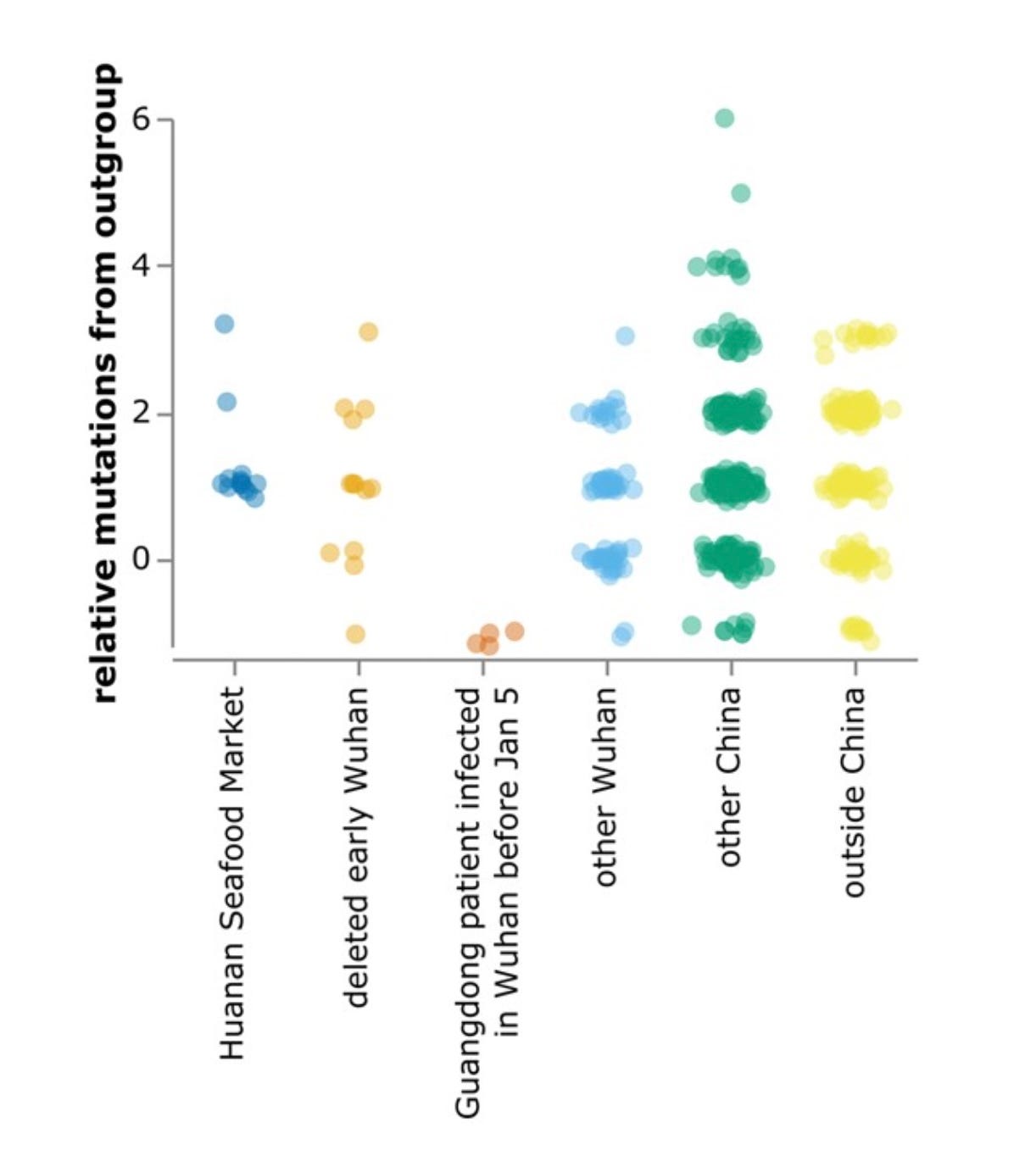
Both Kumar et al. and Bloom have analyzed the phylogenetic data, concluding that the MRCA was, if not A itself, likely to differ from A by an additional nt shared with wild relatives but not with B. (There is some reason to doubt that conclusion since A differs from the main suspect by a T→C mutation, much less common at this stage than a C→T mutation, although non-reversionary mutations are much more common than reversionary ones.) Bloom notes that cases were already being reported by mid-November 2019 and Kumar et al. estimate that the MRCA was probably present in Oct. 2019, with the first spillover case likely to have occurred weeks earlier. A later analysis from the Kumar group using updated techniques and more complete data places the date “in mid-September to early-October 2019”. Bloom finds more early lineage A at multiple locations away from the market, including other parts of Wuhan, other parts of China, and other countries, as seen in his Fig. 4, reproduced below. The phylogeny data thus seem inconsistent with HSM being the only spillover site, since a lineage closer to the ancestral relatives was spreading widely around the time the less-ancestral lineage showed up at HSM.

A thorough new [Chinese paper on the phylogeny issue](https://academic.oup.com/ve/advance-article/doi/10.1093/ve/veae020/7619252?login=false) that uses the most complete data came out in early 2024. The Zhang group finds no evidence of discontinuous evolution, i.e. they found clean sequences that are intermediate between A and B. Their existence tends to undermine the premise of Pekar et al. although it does not prove that the intermediate sequences were upstream of B. They conclude, contra Pekar, that a single spillover is most likely. (As discussed in the Appendix, the same [conclusion follows even without those sequences](https://arxiv.org/abs/2510.01484) just from fixing explicit math errors in the Pekar et al. paper.) They find four plausible candidates for the MRCA, including the two Bloom pointed to, one of which is also the one preferred by Kumar et al. They write “In sum, although multiple lineages of SARS-CoV-2 were co-circulating during the early period of the COVID-19 epidemic, they still exhibited the evolutionary continuity. All of them may have evolved from one common ancestor, probably lineage A0 or a unidentified close relative, and jumped into human via a single zoonotic event.” No version of lineage B is included as a plausible MRCA. MATHPH4XEND
A [paper by Samson et al.](https://journals.plos.org/plosone/article?id=10.1371/journal.pone.0301195) now uses a more complete data set to estimate the spillover time via the MRCA giving a value “between August and early October 2019”. (A peculiarity in one figure, showing RATG13 as descended from an ancestor dated after RATG13 was reported to be sampled, is a reminder of the perils of taking these analyses too seriously.) The later part of that range agrees generally with the estimates from the Kumar and Bloom groups, although the 2022 Pekar model and others referenced in it based on more limited data sets estimate a later time.
At any rate, the MRCA timing does not settle the question of whether the MRCA was in a human or only in some prior natural or lab host followed by more than one spillover. Data on early human cases is more relevant, but as we shall see they aren’t completely clear-cut.
Although the possibility of artifacts cannot be excluded, [La Rosa et al. found wastewater evidenc](https://www.sciencedirect.com/science/article/pii/S0048969720352402?via%3Dihub)e that SC2 started to show up substantially in northern Italy by December 18th 2019. ([Fongaro et al](https://www.sciencedirect.com/science/article/pii/S0048969721012651?via%3Dihub#bb0090). found positive wastewater test for November 27 in Brazil, although probably from contamination since there were mutations that only appeared later than that.) If the seemingly careful Northern Italy report is correct the spillover would have had to have been more in the range estimated by the Kumar and Bloom groups rather than the late estimate of the 2022 Pekar paper.
There were many reports from [Western experts of hearing of the new coronavirus well before the few initial HSM cases](https://ianbirrell.com/leading-us-scientist-i-was-told-about-the-wuhan-outbreak-two-weeks-before-beijing-warned-the-world/) could have triggered reports. A [published report in National Geographic](https://www.nationalgeographic.com/science/article/this-globetrotting-doctor-saves-lives-by-diving-into-hot-zones) also indicates that SC2 was becoming widespread in Wuhan by November 2019: “In early January, when the first hazy reports of the new coronavirus outbreak were emerging from Wuhan, China, one American doctor had already been taking notes. Michael Callahan, an infectious disease expert, was working with Chinese colleagues on a longstanding avian flu collaboration in November when they mentioned the appearance of a strange new virus. Soon, he was jetting off to Singapore to see patients there who presented with symptoms of the same mysterious germ.” Likewise, the prominent Dutch viral gain-of-function researcher R. Fouchier reported (see 1:50 [here](https://www.youtube.com/watch?v=5DeUBLeMnjY)) hearing of the new outbreak in the first week of December, 2019.
Data from several search engines also indicate early spikes in interest in some SARS-like infection. On Dec. 1-3 2019 there was a particularly noticeable spike in searches for “SARS” [on the Chinese WeChat si](https://mhealth.jmir.org/2020/10/e19589)te, apparently representing thousands of searches. Other [early blips from Chinese cities](https://www.psychologytoday.com/intl/blog/long-fuse-big-bang/202005/mysterious-blips-raise-questions-about-covid-19-timeline) do not have publicly quantified absolute magnitudes.
The earlier time estimated from these other lines of evidence is inconsistent with the account in which cases start with a spillover at HSM in early December 2019. I do not use that as evidence against the HSM account because the sequence-based timing estimates have big uncertainty and the other evidence isn’t quite airtight.
The point of the Pekar et al. paper seems to have been that the absence of traces of early lineage A in HSM does not rule out the possibility that HSM was a spillover site for lineage B since lineage A could have spilled over elsewhere or perhaps also at HSM but leaving neither detected cases nor early-case RNA there. That possibility does not require that the probability of having had just one spillover is very small, just that the probability of having had more than one is not very small. Thus although the many errors in the Pekar et al. paper, discussed in Appendix 2, invalidate its conclusion that a unique spillover was highly improbable the lineage results are still at least somewhat compatible with a multi-spillover picture including one at HSM.
We’ve looked at whether the sequences found in the HSM were reasonably compatible with that being the only spillover site (they weren’t) but we haven’t made the equivalent test for WIV. Depending on what sequences were there, one could end up with a Bayes factor either favoring ZW or LL.
We know that the [DEFUSE](https://s3.documentcloud.org/documents/21066966/defuse-proposal.pdf) proposal claimed WIV had more than 180 relevant coronavirus sequences, apparently including [many unpublished ones](https://www.youtube.com/watch?v=m96My1v23wM&t=2359s) MATHPH5XEND. Unfortunately we have little information about those. Publication of newly gathered sequences seems to have abruptly stopped with those gathered in early 2016, [according to the data I’ve been provided](https://docs.google.com/spreadsheets/d/1Aa549h5vUfvnZ-PTTNGviDWF1bsTo769/edit?usp=drive_link&ouid=106543307891005183746&rtpof=true&sd=true). In Sept. 2019 [WIV started removing public access](https://www.researchgate.net/publication/349073738_An_investigation_into_the_WIV_databases_that_were_taken_offline) to its sequence collection, finishing early in the pandemic. [Daszak has now conceded in Congressional testimony](https://twitter.com/emilyakopp/status/1785704622197260358) that WIV continued gathering samples after the last reported ones. Daszak [further conceded](https://www.science.org/content/article/house-lawmakers-both-sides-grill-head-nonprofit-worked-with-chinese-virologists) )
Levin has now done extensive modeling of the early case home addresses combined with the approximate case times. This allows the use of more conventional modeling methods for infectious disease spread. Focusing on modeling the unlinked cases, he finds a Bayes factor of 27 favoring a spillover from research on the south side of the Yangtze over spread from the HSM. I suspect there maybe a missing factor favoring ZWM, however, because the model seems to assume that an HSM-linked cluster is to be expected under LL. While we have seen, based on other cities, that it is not extremely surprising under LL it certainly has a probability less than 1. Roughly speaking, at least for now, the combined case home-address-time data do not give a clear Bayes factor favoring either ZWM or LL. That conclusion may change with further modeling, but as we shall see unless it changes substantially ZWM will already be disfavored over less specific ZW versions.
Worobey et al. present another argument— that the distribution of SC2 RNA within HSM pointed to a spillover from some wildlife there. If correct, that argument would be more directly relevant to whether a spillover occurred at HSM than are the locations of selected cases after Covid became more widespread.
The positive SC2 RNA reads did tend to cluster in the general vicinity of some of the HSM wildlife stalls, even after correcting for the biased sampling that focused on that area. That area, however, is also where bathrooms and a MahJong/cards room are located, both likely spreading sites. Demaneuf documents evidence from several Chinese and Western sources that the early market cases were largely of old folks who frequented the stuffy little crowded games room. A finer-grained map using the Worobey data and their heat-map method (reproduced below) showed the hot spot for the proportion of samples that test positive to be centered on the bathroom/games spot, although one wildlife stall is also close by. (Zach Hensel reports that there’s also another right next to the bathrooms, although the Worobey paper only shows an “unknown meat” stall rather than another live animal stall.) Here the bathrooms are shown in green and the wildlife stalls in brown.
As we have seen, even the lead author of Proximal Origin thought having an FCS was at least some evidence favoring LL. Nevertheless, the argument that simply having an FCS gives a major factor is exaggerated, since it would only apply to some generic randomly picked relative. SC2 is not randomly picked. We are only discussing SC2 because it caused a pandemic. So far as we know having an FCS may be common in the subset of hypothetical related viruses that are capable of causing a human pandemic. In other words even though for some generic sarbecovirus P(FCS|ZW) is much less than one, P(FCS|ZW, pandemic) need not be. One needs to be cautious in using fitness-enhancing features such as the FCS in likelihood calculations because of this observational selection bias issue. (See Appendix 4 for a consolidated discussion of how the FCS data are used here.)
Although it is not appropriate to use the non-existence of FCS’s in bat sarbecoviruses to estimate P(FCS|pandemic, ZW) the lack of an FCS in any non-bat sarbecoviruses may provide weak evidence that even though an FCS can enhance fitness in respiratory infections it’s just hard for sarbecoviruses to acquire one. The FCS of SC2 clearly has provided major evolutionary advantages for transmission in other species, yet there are no other known FCS-containing sarbecoviruses in any of the non-bat species known to host sarbecoviruses. The long period of bat interactions with a range of other non-bat mammals has not produced a spillover of a persistent FCS-containing virus even though it has produced a few successful spillovers to non-bats, specifically two pangolin species, raccoon dogs, palm civets, and incidental spillovers to wild boar and ferret badgers. The infection in at least pangolins has similar lung symptoms to that in humans. One might expect each successful non-bat sarbecovirus to have higher probability of having an FCS than would a recently spilled-over human sarbecovirus, even one that was to go on to later have a successful career as a pandemic-causer, since these non-bat viruses have had more chances to pick up an FCS, especially by template switching with host DNA, than the undetected hypothetical intermediate natural ancestor of SC2. There should be a factor disfavoring ZW based on this empirical lack of sarbecovirus FCS’s even in the face of selection pressure, but given how few spillovers there have been outside bats, for now I’ll not draw any separate factor from this although the presence of the FCS struck everyone from Andersen to Baltimore as suggesting lab modification.
L5 = 0.0.
This dummy factor is left in as a marker of a mistake in an earlier version, in which I didn’t realize that most of the non-bat cases were derived from SC2. If one treats SC1 and the several non-bat sarbecoviruses (especially the pangolin version with human-like respiratory symptoms) as representing zero FCS’s on several tries one would obtain an odds factor of 2 or 3 (logit of ~1) favorable to LL. (I’m leaving that out partly out of embarrassment at having mistakenly over-estimated it before.)
The specific contents of the FCS, may also provide evidence. Focusing on the internal details of the FCS site is not cherry-picking statistical oddities from a large range of possibilities, since it is specifically the tiny FCS insertion that seems so peculiar for this type of virus and so predictable for DEFUSE-style synthesis. One of the Proximal Origin authors, Robert Garry, initially reacted: “ I really can’t think of a plausible natural scenario where you get from the bat virus or one very similar to it to \[SC2\] where you insert exactly 4 amino acids 12 nucleotide that all have to be added at the exact same time to gain this function – that and you don’t change any other amino acid in S2? I just can’t figure out how this gets accomplished in nature. Do the alignment of the spikes at the amino acid level – it’s stunning. Of course in the lab it would be easy to generate the perfect 12 base insert that you wanted.” One particular detail of the FCS (codon usage, discussed below) initially struck David Baltimore as a “smoking gun” for LL, although he later moderated that claim.
The feature that struck Baltimore is that the SC2 FCS has two adjacent arginines (Arg’s), each coded for by the nucleotide codon CGG. CGG is the least common of the 6 Arg codons in all related natural viruses. CGG is only used for ~2.6% of the Arg’s in the rest of SC2. None of the other 40 Arg’s on the spike protein use CGG. If we treat them as approximately independent we get P(CGGCGG|ZW)= 0.0262 = ~0.0007. One can check the independence assumption for generic sarbecovirus codons using Arg pairs in closely related viruses, finding that there are zero CGGCGG’s of over 3000 ArgArg’s, indicating at best no tendency for CGG’s to pair and perhaps a tendency not to. In a broader set of relatives (betacoronaviruses), the fraction of ArgArg pairs coded CGGCGG ranges from 0 outside Africa and Asia to 1/10790 in Asia to 1/5493 in Africa.
The probability of finding a CGGCGG in some generic ArgArg pair thus turns out to be very low compared to an estimate of the probability for a synthetic sequence, to be discussed below. The most favorable ZW likelihood then follows a different path, a possibility of which I was initially unaware but which a pseudonymous twitter user, “Guy Gadboit”, pointed out to me. (Gadboit will appear later with some useful simulations.) The pattern that Garry noted could be typical for a lab insertion but could also occur by a one-step natural insertion of the whole 12 nt piece. Such large insertions are not common, but when they do occur they have different codon frequencies than the rest of the virus since the insertion can be read in a different frame than the source, can be reversed in direction, and has different nucleotide frequencies. Fortunately, an initial tabulation of the fraction of ArgArg’s that would be coded CGGCGG in such random long insertions in a collection of related coronaviruses has been calculated by Gadboit to be 0.0227 (14 of 616 potential ArgArg codes in inserts found at least twice), much larger than the values estimated from the rest of the sequence or from actual ArgArg coding in related viruses. (Gadboit’s more inclusive count, not requiring that an insert appears more than once, is 74/4970=0.0159.) Since the appearance of the extra 12nt piece already strongly suggested that it was a recent long insert, there is no need to reduce the 0.0227 much to allow for other possible evolutionary paths. We have ln(0.0227 )= -3.8, with fairly small uncertainty, say ±0.7, i.e. a factor of 2. This should be taken as an upper limit since to the extent that some more protracted evolutionary path were involved one would expect the CGGCGG probability to relax partway back toward the very small net average value.
Although the indications that the FCS is a single-step insert boost P(CGGCGG|ZW, insert) compared to P(CGGCGG|ZW), important mutations do not usually occur via single-step inserts. Early discussions of the possible FCS evolution by proponents of zoonotic accounts do not include the insert pathway. Thus I should in principle include another factor P(FCS via insert|ZW)/P(FCS|ZW), further reducing P(CGGCGG|ZW). I’m not sure how to calculate that factor but it should somewhat favor LL..
We need to compare P(CGGCGG|ZW) with an estimate of P(CGGCGG|LL). Here the argument will be less direct than for P(CGGCGG|ZW), because we don’t have a good extensive comparison set of lab insertions similar to that hypothesized for FCS under ZW. Since we will have to refine our estimate of P(CGGCGG|LL) using synthetic sequences other than viral inserts, it’s important to consider how the optimization criteria vary for different synthetic purposes and how that might affect codon use. The discussion is tedious so I’ve moved it to Appendix 4.
Given the strong indications that CGG is a popular codon for use in synthetic sequences for human hosts, I’ll assume that the purely random 1/36 is the absolute minimum estimate of P(CGGCGG|LL). As discussed in Appendix 4, there are a couple of plausible though not compelling accounts of why CGGCGG might specifically be chosen. The absolute maximum estimate is of course 1.0. We can then use the geometric mean between those limits as our consensus estimate, 1/6. Using a uniform prior on the log we get ln(P(CGGCGG|LL))= -1.8 ±1.1. Combining with our estimate for ZW gives
L6 = 3.8-1.8 = +2.0
For this term, properly separating the integrals over uncertainties in the two likelihoods would raise the LL ln(likelihood) by ~0.4 and raise the ZW term by ~0.25, giving a net logit ~2.1.
Out of conservatism I’ll slightly break the rule here and just leave it at
logit6 = 2.0
Since the estimate of P(CGGCGG|LL) is pretty fuzzy, this should be taken as conservatively including allowance for the relative likelihood of the FCS arising by a recent single-step insert under ZW compared to that likelihood under LL.This is far less important than the result I had initially used based on whole-sequence codon frequencies.
\[10/19/24. [Gadboit has just analyzed possible bacterial sources of the 12 nt insert](https://drive.proton.me/urls/CFZPVEY4V0#1cEXo9KaMyq5), unsurprisingly finding numerous matches to the 12 nt sequence. He finds that the nts neighboring the 12 nts in these bacterial sequences tend to match those of SC2 at a higher-than-chance level. He suggests that match may facilitate template-switching inserts and thus may be evidence for a bacterial source of the 12nt insert, presumably in a less serious version of SC2 circulating unnoticed in a human population harboring the relevant bacteria. This proposal amounts to a specific form of the earlier one from [Temman et al.](https://pmc.ncbi.nlm.nih.gov/articles/PMC10074129/) of a previously circulating human enteric version. Although there are indications in Cambodia of [serological traces of prior exposure to some viruses](https://onlinelibrary.wiley.com/doi/10.1002/advs.202403503) not too distant from the SARS-related group, [Temman et al.](https://pmc.ncbi.nlm.nih.gov/articles/PMC10074129/) found no serological traces of the pre-FCS SC2 human infection in the suspected regions, so for now this theory seems unlikely to pan out.\]
The DEFUSE proposal mentions plans to modify the N-linked glycans of a natural backbone. Their fitness depends strongly on the host environment. SC2 is missing one that is found in its relatives. Further work would be needed to estimate how much that should change the likelihood ratios. It is particularly relevant for the direct bat to human route, since that would require two features (getting an FCS and losing the N-linked glycan at position 370) that are unfit in bats.
Bruttel, Washburne and VanDongen claimed in late 2022 to have identified in SC2 a pattern of segments that would be defined by cutting with the restriction enzymes BsaI/BsmBI that was characteristic of synthetically assembled coronaviruses. The restriction enzyme pattern is perhaps the most useful of the sequence features because it has nothing to do with natural selection constraints, so its interpretation is relatively simple. It serves as a probabilistic indicator favoring LL over any version of ZW or ZL, including direct-from-bat spillover and accidental acquisition of an FCS by a previously unnoticed human virus.
\[4/8/25\] It now turns out that the National Center for Medical Intelligence, preparing a report for the Defense Intelligence Agency, already noticed exactly this pattern in 2020. The DIA report refers to the “invisible restriction sites”, apparently referring to sites that might have been used for initial assembly. The BsaI/BsmBI sites that Bruttel et al. surmised were left in for use in ongoing substitutions were visible, and shown on the line starting at 1 going to 29903.
Arguments about how much weight to put on anecdotal evidence for or against strong proximity-based ascertainment bias are unlikely to be persuasive to anyone with strong prior opinions. I have noticed, however, that the Worobey et al. paper includes internal evidence that shows rather conclusively that there was major proximity ascertainment bias. The argument that follows is my only original contribution to the origins dispute.
Let’s consider two hypotheses, W and M. W is that all the cases ultimately come from the HSM and that fact accounts for the observed clustering near the HSM, with no major ascertainment bias. M is that the proximity ascertainment bias is too large to allow inference about the original source from the location data. These hypotheses have opposite implications for the correlation between detected linkage to HSM and distance from HSM.
For hypothesis W there is some typical distance from HSM to a linked case. An unlinked case must come from a linkable case (typically not observed) via some additional transmission steps in which the traceability is lost. The mean-square distance (MSD) to HSM of the unlinked cases would then be approximately the sum of the MSD of the linked cases and the MSD of the other steps in which traceability was lost. Given that there are many more unlinked cases and that unlinked cases were at least as hard to detect several such transmission steps would typically be involved. Barring some peculiar contrivance, the unlinked cases are then on average farther away from HSM than the linked cases. The linkage-distance correlation is negative.
For hypothesis M case observation can arise either via linkage or proximity. Some cases are found by following links, others by scrutiny near HSM. Observation is a causal collider between linkage and proximity: linkage→observation←proximity. Within the observed stratum of cases collider stratification bias then gives a negative correlation between linkage and proximity, i.e. a positive linkage-distance correlation.
The relevant observational results are reported clearly by Worobey et. al. “(ii) cases linked directly to the Huanan market (median distance 5.74 km…), and (iii) cases with no evidence of a direct link to the Huanan market (median distance 4.00 km…. The cases with no known link to the market on average resided closer to the market than the cases with links to the market (P = 0.029).” The statistical significance of the deviation from the W hypothesis is even stronger than the “p=0.029” would indicate since that calculation was for the hypothesis of no difference but W implies a noticeable difference of the opposite sign. Thus the W hypothesis is disconfirmed by the data of Worobey et al. The sign of the linkage-distance correlation instead agrees with the M hypothesis, that there is substantial proximity-based detection bias.
Since the reports of the early cases included a claim that there was no evidence of human-to-human transmission, the linked cases must almost all be directly linked with the patients themselves having been at the market. Unlinked cases, in contrast, could easily be more than one transmission step away from their last linkable ancestor. In order to account for the unlinked cases being much more common despite a tendency for the linked to be easier to detect there must be typically at least two post-linkable steps. Although the typical relative displacement of an unlinkable step is not known, that there are typically several such steps strengthens the case that the unlinkable cases should be appreciably farther from HSM than the linked ones if W holds.
More informally under W one would also expect the more distant unlinked cases to be displaced in roughly the same directions as the linked cases from which they descend, since linked cases can spread infections at home and to and from work. Visual inspection of the map of linked and unlinked cases, Worobey et al.’s Fig. 1A, does not support such an interpretation since the more distant linked cases tend to be north of HSM and the more distant unlinked south and east. Quantitatively, using the case location data from their Supplement one finds an angle of 105° between the displacements from HSM to the centroids of the linked and unlinked cases, i.e. a slightly negative dot product between those typical displacements. That would be surprising for any account in which cases start with a linkable market transmission and then at some point lose linkage through an untraceable transmission.
Worobey et al. include kernel density estimation (KDE) contour maps for the unlinked cases and for all the cases. These convey information complementary to the centroids because they emphasize the most clustered points rather than the more distance ones. Daniel Walker has superimposed Worobey’s KDE map of the linked cases (posted on github but omitted from the paper) with their corresponding unlinked map. This map again shows a remarkable tendency of many of the unlinked cases to cluster much closer to the market than do the linked cases, whose main cluster is displaced toward the river.

Worobey et al. do propose a distinction between types of linked cases that could in principle lead to difference in distances between linked and unlinked cases. They point out that home addresses of cases linked because the patient (or a linkable contact) worked at HSM might typically be farther than ones linked via other activities, e.g. shopping at HSM. They do not directly explain how that heterogeneity within the linkable cases would give a distance contrast between linked and *unlinked* cases. In order for that difference to show up as the observed effect one would need to add another assumption, that it would be harder to trace secondary connections to the nearby linked cases. No explanation is given for why such an effect would be expected or for what sign it would be expected to have. One might expect that among people near the market it would be easier to find contacts with neighbors with linked cases. A second-order explanation along these lines remains in the realm of possibility although more speculative than the simple first-order observational collider bias.
Débarre and Worobey have now posted a [reply](https://arxiv.org/pdf/2405.08040) to my paper on proximity ascertainment bias. Essentially, they now dismiss the p-value of 0.029 given in the original Worobey paper for the linked/unlinked contrast. They say that when one takes into account the overdispersion of the SC2 transmission and the possibility that the typical distance between the point of acquiring an infection and passing it on could be less than the typical distance from the point of acquisition to the point of residence, there could be a higher chance of finding unlinked cases closer to linked cases than given by the original p-value. They present some simulations of multi-step transmission to support that claim. They claim that their simulation is conservative because its first step goes from HSM to a residence, before subsequent shorter infection-to-infection steps. Since the step operations commute, however, this is exactly equivalent to a model of infection-to-infection steps followed by a single step to the residence location.
The probabilities they present are for the unlinked median distance being less than the linked rather than for the actual result (a ratio of 0.70) reported by Worobey et al. Jon Weissman has re-run the simulation provided by Débarre to see what p-value it gives for the actual reported data as a function of the ratio of infection-infection distance to infection-residence distances. I.e. he ran the Débarre code with no changes other than using the observed 0.70 ratio rather than an arbitrary 1.0 ratio to calculate the p-value of the observation. (The simulation code used by Débarre and Worobey is peculiar in some respects such as using a probability density function for vector displacement in 2-D that diverges for small displacements, but we leave it unaltered to avoid quibbling about details.) The results are here.
s_!6rgR!,w_1456,c_limit,f_auto,q_auto:good,fl_progressive:steep/https%3A%2F%2Fsubstack-post-media.s3.amazonaws.com%2Fpublic%2Fimages%2F040b9174-2c3a-4c67-91e1-9e3e0af04c9f_1300x650.png)
For the nearly Poisson case (kappa=100) with no infection-infection displacements the p-value reproduces that of the original paper. For the overdispersed case (kappa=0.4) the reported results remain highly unlikely to be consistent with the model unless the typical distance from the place of acquiring the infection to the place of passing it on is less than about 20% of the distance to home. That would not violate any laws of physics but seems quite unrealistic and is unsupported by any evidence.
Further confirmation of the poor fit with a model of unbiased sampling of cases descended from ones that started at the market has been provided by another simple statistical test run by another pseudonymous analyst. The question is whether the contrast between the linked and unlinked case location distributions could result from random sampling. The non-parametric test is to repeatedly randomly divide the 155 Worobey cases into sets of 35 and 120 and compare the average distances in those two sets from their centroids. As with distance from HSM, one would expect that additional transmission steps would increase the spread in the locations around their centroids, but the opposite result is found. “Unlinked cases are an average of 5 km closer to their centroid than linked cases are to their centroid (-5.06 km). The central 95% of the permuted stat is -4.4 km to 3.5 km.” The algorithm is included in Appendix 3. The same analyst noticed that the displacement of the centroids from each other was significantly larger than would be expected for random sorting, but since the unlinked transmission steps could easily have a net average direction that is not evidence against a Worobey-like model.
Some reactions to my JRSSA paper have emphasized that Worobey et al. included a discussion of ascertainment bias in their supplementary material. Most of that discussion is irrelevant to the type of bias that I discuss, and perhaps to other types as well. The bias specific to the unlinked cases is discussed only in the following passage:
“So, could those unlinked cases have been detected via biased case-finding involving searching for cases only in neighborhoods near the market but not in other parts of Wuhan? Not likely. Remembering that all the cases were hospitalized and that no diagnostic test was available to identify mild cases it is likely that most or all Huanan market-unlinked cases were ascertained while in hospitals.”
The argument only applies to the possibility of false positives. The entire issue, however, is not false positives but false negatives. Unlinked cases away from the market appear to have been detected at a disproportionately low rate, just as Bahry, Demaneuf, and others had argued based on statements from Wuhan participants.
Although as we’ve seen the question of whether there were two spillovers or one has little or no general direct relevance to LL vs. ZW, the absence of early sequences of the more ancestral lineage A from HSM fits poorly with the HSM version of ZW unless there were multiple spillovers. Thus despite its limited general relevance a good deal of attention has been paid to the argument of Pekar et al. that there were two spillovers.
Pekar et al. use a Bayesian calculation to infer the probability that there were two spillovers rather than one based on the later phylogenetic pattern. As He and Dunn noted in an eletter posted with the paper soon after publication, the Pekar paper had no model for its two-spill hypothesis and thus could not in principle calculate its likelihood. The most unambiguous logical error of Pekar et al. was to require that the disfavored single-spill hypothesis meet much more detailed conditions than the favored two-spill hypothesis in comparing their likelihoods. It is obviously essential that the same observational features be used for each hypothesis. For example, if one were to update the odds for deciding which of two suspects committed a burglary where a blue Toyota was spotted leaving the scene, it would not be correct to use the ratio P(drives car|suspect 2)/P(drives blue Toyota|suspect 1). That would be a fundamental error in logic, precisely analogous to the Pekar et al. error.
Just correcting that error reverses the odds, making the single-spilled hypothesis favored, even when parameters are adjusted to favor the two-spill hypothesis. Nevertheless, one can set limits on what the likelihood of the two-spill hypothesis would be just using the one-spill model of Pekar et al. Since that issue is now dealt with in an eletter now posted with the paper and, in more depth, in the arXiv paper by McCowan and in Econ Journal Watch by me, I’ll focus on other issues here. The collection of the other errors sheds further light on the quality of work in this area.
As background, three pubpeer analyses by McCowan found multiple errors in the code used to calculate the likelihood ratio. One error seems to be due to a simple copy-paste mistake. The next is somewhat more conceptual, an incorrect normalization of the likelihoods. Together those two “combined corrections reduce the Bayes factors from ~60 to less than 5.” The third is a double-counting error: “Removing the duplicated likelihoods reduces the Bayes factors by a further ~12%.” A numerical correction for these three coding errors has belatedly been included in the Science paper, reducing the claimed Bayes factor from ~60 to ~4.3. The verbal results were not noticeably changed and it was not acknowledged that the errors were discovered by a pubeer contributor. The full story is recounted by Demaneuf.
Thus simply fixing the clear mathematical and programming errors of Pekar et al. leaves N=1 more probable than N=2, a conclusion opposite to the key result proclaimed in the paper. Meanwhile, new data on intermediate sequences tend to undermine the empirical basis of the whole lineage story. To what extent the remaining plausibility of N=2 would survive the remaining corrections is unknown.
Even without finding the simply erroneous mathematical analysis, readers should have been able to see other fundamental problems with the model. The simplifications used in the model have been described as strongly inappropriate for SC2, with arbitrary and likely unrealistic probability distributions of spreading events, including the omission of the abrupt single-time superspreading events that tend to generate the polytomies whose analysis forms the core of the Pekar analysis. As S. Zhao et al. wrote, Pekar et al. miss other fundamental ingredients: “In the coalescent process of their simulations, they assumed that viruses spread and evolve without population structure, which is inconsistent with viral epidemic processes with extensive clustered infections, founder effects, and sampling bias.” Omitting the blotchy population structure of transmission and blotchy ascertainment probability in location and time severely loosens the connection between the model and real data.
Since having a non-ascertained early phase in a distinct population (other host species) introduces just the sort of realistic elements that were left out of the over-simplified model, making the model more realistic should increase the likelihood more for N=1 than for N=2. In other words, the phylogenetic pattern noticed is the failure to find early sequences intermediate between two later batches separated by 2nt. The absence of intermediates from the limited data set could be ascribed either to their having occurred in some unobserved previous host species or to the known strongly reduced early ascertainment probability in humans.
The Bayesian priors used by Pekar et al. are peculiar even on superficial inspection. Oddly, after much complicated error-prone model-dependent analysis of the likelihood ratio for two spillovers vs. one spillover the Pekar et al. just arbitrarily assigned prior odds to be 1.0. (See page 13 of the Supplement to Pekar et al.) In effect the prior probabilities they used for the number of successful spillovers, were P(1) =1/2, P(2)=1/2, P(3)=0, P(4)=0, etc. Let’s assume, pretty realistically, a Poisson distribution for N with expectation value x. There is no value of x nor is there any probability distribution of x that leads to the set of prior probabilities use by Pekar et al. Thus it looks like a post-hoc attempt to inflate the prior probability of N=2.
We don’t know x but it can’t be very small because then no spillovers would have been found or very big because then even more than two would have been found. A standard non-informative form for the prior probability density function of x is 1/x. Since we require N>0 to observe a pandemic the probability density of x for observed cases excludes the N=0 cases, leaving a distribution of the form (1-e-x)/x, eliminating the small-x divergence of the integral. Its integral diverges weakly for large x but that divergence will not affect the odds. We can then easily integrate the Poisson probabilities over x to get the prior odds, P(N=2)/P(N=1) = 1/2. (Extension of this method to higher N gives a very weakly divergent sum of probabilities that stays finite if truncated, e.g. at N= population of Wuhan.) These conventional non-informative priors would reduce the resulting posterior Bayes odds by another factor of 2. It is peculiar that the paper did not use such a conventional exercise to obtain the prior odds without post-hoc adjustment.
This model automatically shuts down the spillovers after two have occurred. For a large host population, that would not be close to realistic since the infection would spread approximately exponentially, leading to far more spillovers later. A lab in which containment measures are taken fairly soon after a spillover is noticed could easily fit the model. Transmission from a small pool of infected animals in one or two markets might also fit, though not as easily. Transmission from a disease spreading in some larger animal pool would run into qualitative problems accounting for the small number (probably one) of spillovers.
This conclusion does not necessarily lead us to change our P(LL)/P(ZW) odds much. It does, however, further weaken the case for the particular HSM version of ZW, since the N=2 hypothesis was used to plug the hole created by the absence of the more ancestral lineage in the market-linked cases.
With regard to the MRCA, Pekar et al. point out that most reversionary mutations are of the C→T form, regardless of which MRCA is picked. 19 distinct such mutations were found in the 787 early sequences they describe. Only 4 other distinct reversionary mutations from lineage B were found, or 3 from lineage A. The C→T mutations often showed up more than once; I count 41 times in their Figure 1. Non-reversionary mutations also occur more than once, with the total mutation count running about 1000, since many sequences descend by multiple mutations from their closest ancestor. Since lineage A differs by a C→T and one other, coincidentally T→C, if we confine the possibilities to either B descended from A or A from B, the odds for B from A are P(non-reversionary (C→T & other))/P(reversionary (C→T & other)). Using that C→T mutations account for roughly half of all the mutations, this ratio becomes about (1/2)(1/2)/((1/25)(1/250)) = ~1500/1. This result is slightly larger than what we found without distinguishing between different types of reversions or considering the frequencies of each type. Thus following Pekar et al. to distinguish between C→T and other reversions supports the case that a pure B spillover is highly improbable.
One sequence listed (MKAK-CL-2020-6430) differs from B by only 4nt, all reversionary, 2 C→T’s and 2 others. The probability that if B were the MRCA any of the 787 early sequences shown would have a difference of that sort is in the ballpark of
787*(4 choose 2)(41/1000)2(4/1000)2 = ~1.510-4. Even allowing for the post-hoc choice of features, i.e. some potential multiple comparisons, this is a low probability. If lineage A were the MRCA, the expectation value of the number of sequences meeting those criteria would be ~787*(2 choose 1)*(41/1000)(4/1000) = ~0.3, so finding one would be entirely unremarkable.
Once again, including Pekar et al.’s emphasis on the special role of C→T reversions makes a pure-B spillover even less plausible. Although their case for a high probability of two spillovers disintegrates under inspection, the current phylogenetic analysis only says that two spillovers have a moderately low probability, not enough to downgrade the possibility of an HSM spillover much further. The tiny fraction of the wildlife trade that went through Wuhan gives a much larger factor without any subtle complications.
Pekar et al.’s reversion statistics also help make the Sangon sequences more interesting. The probability that of the 14 Sangon mutations (relative to lineage B) at least 2 would be C→T reversions and at least 1 another reversion is only ~1%. (If any are just misreads, that percentage drops further.) The probability that those 3 reversions would exactly match the Kumar MRCA rather than other 20 known early reversions is of course lower, somewhere in the vicinity of 10-5 if each C→T is equally likely as is each other reversion. That dramatic match cannot be fully explained simply by saying that the earliest mutations determined Kumar’s choice of MRCA since in order to avoid distortion from time-dependent ascertainment probability the Kumar modeling explicitly did not use the observation dates of early sequences. The presence of these mutations in the small set from these early samples seems inconsistent with a unique B spillover.
In an article in the influential political journal Foreign Affairs, Rasmussen and Worobey described the Pekar et al. results as “we find a roughly 99 percent probability that SARS-CoV-2 spilled over at least twice”. The first published version of Pekar et al. had the chance of fewer spillovers at ~1.6%. By the time the first batch of coding errors were acknowledged, the published chance had gone up to ~19%. Nod’s rerunning that code enough times to get good statistics gave ~23%. Correcting the most blatant imbalance in the outcomes used for the conditional probabilities then raised that to ~63%. Correcting the remaining imbalance using parameters adjusted to maximize the probability of the two-spillover hypothesis raises that to ~ 81%. 81% chance of being wrong is a lot different from ~1%. So far as I know, Foreign Affairs has published no erratum.
A talk by Worobey repeated the Pekar et al. errors and added an additional fundamental one. He described their calculated probability of two spillovers as having been 99.5%, i.e. 200/1 odds. Actually the published paper itself, on which he was a coauthor, had originally given 60/1, with his 200/1 apparently coming from just using one likelihood rather than from taking a ratio, a truly fundamental error. He then corrected those odds to 30/1, i.e. acknowledging the factor of 6 copy-paste coding error but not even correcting the other two coding errors that he and his coauthors had acknowledged. Worobey stuck with the fundamental misunderstanding of how to get odds from likelihoods. He included no acknowledgement of the fundamentally unbalanced outcome requirements used for the two hypotheses, much less for the peculiar priors or the major modeling flaws. In the bulk of the talk, focusing on location data, no mention was made of the evidence undermining the argument for or even contradicting the HSM account.
This talk is important not for our odds calculation but rather for understanding the level of alleged science underlying the canonical account. Whatever may become of my odds estimates in the light of new evidence and new reasoning, the conclusion should hold that the key arguments on which the zoonotic view currently rests are shoddy at best.
The calculations here are not intended to imply unrealistic precision. They are meant simply to use defined logical algorithms to avoid unnecessarily adding even more subjective steps.
To estimate the expected ln(likelihood) and its variance for an event based on observing it M times out of N trials, I subjectively assume a uniform prior on the probability, x, for not finding a host when there actually is one, giving analytically solvable integrals:

For N=2, M=0 we get <ln(likelihood)> = -11/6 =~-1.83 with standard error of 1.17.
For N=4, M=1 we get <ln(likelihood)> = -1.28 with standard error of 0.68.
For N=6, M=2 we get <ln(likelihood)> = -1.09 with standard error of 0.51.
For N=7, M=2 we get <ln(likelihood)> = -1.22 with standard error of 0.53.
(I just found out that this particular exercise is close to the first posthumously published example worked out by Bayes.)
Here’s a description from the author of the test on linked vs. unlinked case clustering. Only the second of their statistics is directly relevant to the selection bias issue.
> Load a CSV from Worobey et al into R as data.frame called “cases.” Compute first stat as: with(cases, distm(c(mean(longitudeMATHPH26XEND), mean(latitudeMATHPH27XEND)), c(mean(longitudeMATHPH28XEND), mean(latitudeMATHPH29XEND)), fun=distHaversine)).
> I ran the permutation test 10000 times. Replace “huanan\_linked” with “assign” for permutation test (random assignment of pooled cases into linked & unlinked as defined above). Use something like quantile(perm\_results, c(.025, .975)) to get central 95% interval under null.
>
> For the second stat, I defined a helper function because we need to run distm to compute the distances of all cases from their group’s centroid and then take the average.
>
> The second statistic is operationalized as: with( cases, mean(compute\_distances(cbind(longitude, latitude)MATHPH30XEND, c(mean(longitudeMATHPH31XEND), mean(latitudeMATHPH32XEND)))) # continues in next reply…
>
> \- mean(compute\_distances(cbind(longitude, latitude)MATHPH33XEND, c(mean(longitudeMATHPH34XEND), mean(latitudeMATHPH35XEND)))) ) As before, replace “huanan\_linked” with “assign” for the permutation test.
For the restriction enzyme segment pattern I tried a quick sanity check on the probability of randomly getting Nseg=6 with maxL<8knt by assuming a Poisson distribution of the number of sites (Nseg-1) with locations drawn independently from a uniform distribution. Fine-tuning the expectation value of Nseg to 6 gives a Poisson probability of 0.175. For the probability of then getting small enough maxL I wrote a simulation R program:
\> for(j in c(3:10)){tot=0
\+ for(i in c(1:1000000)) {vx=sort(runif(j,0,1))
\+ if(max(c(vx,1)-c(0,vx))<0.268){tot=tot+1}
\+ i=i+1}
\+ j=j+1
\+ print(c()
There is no reason to think that this weighting procedure is optimal for a general case, but it’s adequate for the fairly small corrections needed here in our crude model.
\[Jamie Robins has pointed out that the correction used for uncertainty here is formally correct under some simplifying assumptions if the nuisance parameter for each observation is shared between the likelihoods for the two hypotheses. Usually it would be more realistic to treat the nuisance parameters for each hypothesis as independent so that the integral should be done on each likelihood rather than than on the ratio. I’ve now incorporated that change.\]
For small Vi the result is only weakly sensitive to the form of the distribution of qi. To lowest order in Vi the effect becomes logiti = Li -0.5 Vi tanh(Li/2)). For large Vi that lowest-order approximation overstates the correction but the result can be obtained directly from the integrals if a form is assumed for f(qi), e.g. Gaussian or uniform. For a uniform distribution there’s an analytic expression,
ln(ln((1+e(L+s3^0.5) )/(1+e(L- s3^0.5)))/ ln((1+e(-L+ s3^0.5))/(1+e(-L- s3^0.5)))). For the CGGCGG factor I used the same uniform distribution described in the text.
For the last step we combine the prior distribution with the log of the net likelihood ratio, L, the sum of the likelihood logits, to obtain the odds.

To reiterate, our method of taking uncertainties into account *reduces* the odds favoring LL, both for uncertainties in likelihoods and for uncertainty in the priors.
How much does our conclusion that SC2 was almost certainly from a lab change the odds we would give if a similar situation were to show up in the future? We started off with ~70/1 odds favoring some sort of ZW story, but we were quite uncertain about that. We had logit0 =4.2±2.3. Now we can treat that as a continuous distribution of hypotheses about what the best prior odds should have been, expressed as a distribution on x, the log of the odds. We re-evaluated that distribution in light of an observation, using that usual Bayesian likelihood ratios. The observation is our the conclusion that SC2 came from a lab. The very small chance that it didn’t will have negligible effect on the resulting calculation, which is obviously very rough anyway.
For any x the likelihood P(LL|x) remains 1/(1+e\-x). Then
s_!rfnn!,w_1456,c_limit,f_auto,q_auto:good,fl_progressive:steep/https%3A%2F%2Fsubstack-post-media.s3.amazonaws.com%2Fpublic%2Fimages%2F1c4e2985-90e4-4b32-b233-f3ef96ce7c6a_650x228.png)
Let’s recognize the limits of our knowledge by using for the prior our fat-tailed 3-d.o.f. t-distribution with mean of -4.2 and s of 2.3 that allowed a chance of ~1/300 of ZW:

Simply plugging that into the integral gives a posterior distribution for x with mean of -0.50 and s of 3.1. The starting prior and the one to use next time are illustrated here, with the new one on the right. The x-axis is the natural log of the odds.
s_!noyl!,w_1456,c_limit,f_auto,q_auto:good,fl_progressive:steep/https%3A%2F%2Fsubstack-post-media.s3.amazonaws.com%2Fpublic%2Fimages%2Ff93b0079-a047-4593-a9a0-ebf64f5227b2_826x539.jpeg)
The FCS appears at several points in the argument, so it may help to clarify in what ways it is used and in what ways it isn’t used.
Although some have argued that having an FCS is very unlikely for sarbecoviruses since only SC2 has one, that low likelihood may not apply when one remembers the precondition that we wouldn’t be discussing this virus if there weren’t a pandemic for which the FCS may be nearly needed. Only a few non-bat species are known to host sarbecoviruses so it is hard to estimate the probability that a successful respiratory one would have an FCS..
Deigin points out that FCS in SC2 occurs exactly at the S1/S2 junction, an obvious place for a DEFUSE-style insertion. A recently released early draft of DEFUSE (before compression to meet space limits) specifically mentions the S1/S2 boundary as a target for a cleavage site insertion, by sequence location number rather than by name. Since that is also, not coincidentally, an evolutionarily advantageous location, it might only provide a small update factor favoring LL, which I don’t use.
The S2 neighborhood of the FCS, differing from related viruses only by synonymous mutations, has been cited as evidence for LL because it looks peculiar under ZW but not under LL, as noted in the Garry quote above. The initial post-spillover strains lacked a mutation called D614G that becomes advantageous specifically to compensate for some effects of the FCS. D614G arose quickly to predominate in multiple lines of SC2 as it spread in humans. The combination of the FCS coding described below, the lack of amino acid changes in S2, and the initial absence of D614G all indicate that the outbreak started not very long after the FCS was inserted, whether naturally or in a lab.
The picture of a quick route to human spillover after FCS insertion is easily consistent with LL. It fits well with only a particular subset of the zoonotic hypothesis. I don’t use that for an update to avoid partial double-counting with related FCS factors.
The detailed contents of the FCS, the CGGCGG sequence, provide one significant piece of evidence used, since it seems P(CGGCGG|LL) is larger than P(CGGCGG|ZW). On the fuzzy issue of what codons to expect in a synthetic sequence, if the LL codon choice for ArgArg were purely random, we’d have P(CGGCGG|LL)=1/36. When sequences are synthesized for use in hosts, however, they are typically “codon optimized”, using the more common host codons, such as CGG in humans, even more frequently than they are found in the host. CGG codes for 20% of human Arg. Thus a reasonable first minimum estimate of P(CGGCGG|LL) would be 0.22=0.04. More likely, since the two rarer codons would generally not be used, a good low estimate would be (1/4)2=0.063.
I found two convenient relevant examples of how often CGG would be used in modern RNA synthesis for human hosts, specifically of stretches coding for portions of the SC2 spike protein used in the Pfizer and Moderna vaccines. Both mRNA vaccines and viral genomes need to be stable in the host organism and to work well at highjacking the host machinery to generate the proteins for which they code, so there’s quite a bit of overlap in the criteria used in choosing codons.
Unlike vaccine mRNA, however, viral RNA also needs to replicate well and to pack well into the viral package. For our purposes, looking at just a few nt on an insert that already disrupts the previous RNA structure, packing is probably irrelevant. Is there any indication that CGG is thought to be a particularly poor replicator in humans, in which case we should lower our estimate of P(CGGCGG|LL) compared to what’s found in mRNA vaccines? In the years since SC2 started, almost all strains remain CGGCGG, although some synonymous mutations to CGUCGG are now present. Thus there is no indication that a viral sequence designer would have any special reason to avoid CGG for reproductive reasons, so the vaccine coding can give us a rough idea of how likely a CGGCGG choice would be for a synthetic viral sequence.
CGG is used far more often in the Pfizer and Moderna vaccines than in the natural viruses: “The designers of both vaccines considered CGG as the optimal codon in the CGN codon family and recoded almost all CGN codons to CGG.” 19 of 41 Arg codons in Pfizer are CGG, as are 39 of 42 in Moderna. The designers were not inspired to use CGG by its appearance in the FCS on the target protein, since none of the other 40 Arg’s on that protein use CGG. Deigin has pointed out another reason that a researcher inserting coding for ArgArg might specifically choose CGGCGG— it provides a marker for a standard, easy, restriction enzyme test allowing the researcher to know if that insertion is still present or has been lost, an important consideration since FCS’s tend to get lost in cell culture. (AGGCGG would also code for ArgArg and work for the marker.) On the other hand, although both designers were fond of CGG, neither used CGGCGG for the ArgArg pair, indicating that they had some reason to avoid it, perhaps connected to occasional translational errors that might be particularly important to avoid in vaccines although less important for viral fitness. The |LL) likelihood factor here may go up or down if I can track down why the vaccine designers chose not to use CGGCGG.
The amino acid sequence of the SC2 FCS is identical to a familiar human amino acid sequence that would be a good candidate for use in a furin cleavage site promoting infectivity. In that human FCS sequence the ArgArg pair is coded CGUCGA, which would become CGGCGG either under the choice CGN—>CGG usually used by vaccine coders or to implement the standard tracing procedure described by Deigin.
In the one example of which I’m aware in which a collaborator of the WIV group added a 12nt code for an FCS to a plasmid (reminiscent of the 12nt addition in SC2) they only used CGG for one of its three Arg’s. Other plasmid primers from WIV use high fractions of CGG, including CGGCGG dimers, but again these are for plasmid work and thus subject to substantially different optimization criteria.
We can check that we have not missed some important argument that CGG would be disfavored in a lab by reading Andersen’s extensive argument that CGG did not indicate LL. While presenting detailed non-statistical scenarios of how CGG might possibly arise naturally, it makes no mention of any reasons why it might be disfavored in a lab.
Wuhan is not the only place where pathogen research is done, so a priori it would be an exaggeration to say P(Wuhan|LL, pandemic) = ~1. However, the combination of the DEFUSE proposal to add an FCS to coronaviruses, along with other DEFUSE proposed features found, strongly indicate that if SC2 originated from a lab, it would be one doing the DEFUSE-proposed work. The site mentioned in DEFUSE for adding an FCS to a coronavirus, UNC, is smaller and uses highly enhanced BSL-3 protocols. After DEFUSE was not funded, switching this part of the work to WIV, where there was already expertise in the methods, would have been easy. A note from a lead investigator, Peter Daszak, to the NIH about earlier work had assured them in 2016 that “UNC has no oversight over the chimera work, all of which will be conducted at the Wuhan Institute of Virology.” Notes from DEFUSE investigators have recently been released describing plans to actually conduct much of the research described as planned for BSL-3 at UNC instead in Wuhan, where BSL-2 was often used. While the chance of a spillover occurring at UNC isn’t zero, it’s much lower than for WIV. Thus
P(Wuhan|LL, coronavirus with FCS, etc.) = ~1.
So far I have just ignored the ZL account of a virus that formed naturally but successfully spilled over into humans via research activities. For origins via an intermediate host including ZL would just add another research channel increasing the lab vs. zoonotic odds. The sequence evidence indicates that some modification probably occurred in the lab, so including ZL wouldn’t change those odds much. Although the likelihood factors from the FCS coding and the restriction enzyme pattern strongly favor lab modification, it’s worth having a quick look at the P(ZL)/P(ZW) odds for accounts lacking an intermediate host, especially since there’s some chance that SC1 lacked an intermediate host.
Several of the features that we have noted could fit together in a zoonotic picture qualitatively different from the bat—>wildlife—>market—> human version usually considered. The evidence described in Appendix 4 requires there was only a short interval between the FCS insertion and the spillover, perfectly consistent with LL but perhaps also with a particular zoonotic account along the direct-from-bats lines that Wenzel proposed for SC1.
The reports of Laotian BANAL bat sarbecoviruses with good human ACE2 binding but lacking an FCS suggest a way for getting good preadaptation while skipping intermediate wildlife hosts altogether. Someone in or near Laos could have become directly infected with a BANAL-related bat virus that contained a small trace of FCS variants, too little to detect in consensus sequencing tests, before those variants were lost due to their lack of fitness in bats. Likewise an accidental FCS insertion could have occurred in the person before the virus was eliminated. With some luck, the virus might survive long enough for those few FCS-containing virions to become the main strain in the human host. The disintegration of the evidence for an HSM spillover would not be surprising in this zoonotic story, since HSM would have no initial role to play.
Direct-from-bat accounts (whether natural or via research) require wending an especially narrow path to spillover, needing an FCS insert and a properly ablated N-linked glycan to appear almost simultaneously in a virus that already happened to have an RBD well-adapted to humans. The absence of any FCS-containing sarbecoviruses in any host species, including humans, indicates that such coincidences would be rare. It would be worth further investigating the occasional successful spillovers from bats. Thus I do not think that a direct-from bats version of ZW is nearly as probable as the LL one that there was a leak from DEFUSE-like work, perhaps being done using a BANAL-related pre-FCS backbone.
If a direct spillover from a bat or an unmodified sample from a bat did nonetheless occur, the remaining issue would then be how the virus got from Laos or nearby to Wuhan without leaving a trace. This is where ZL accounts become most relevant.
For P(ZL)/P(ZW) odds we can start with Demaneuf and De Maistre’s analysis, predating DEFUSE and some other relevant evidence. Their base estimate, using their best estimates of lab leak probabilities and non-research probabilities, was
P(ZL|Wuhan)/P(ZW|Wuhan) = ~4. They also include a conservative estimate, 1.2, using factors tilted toward ZW compared to their best estimates and a “de minimis” estimate using the most extreme estimated factors, giving 1/15. Rather than reproduce the whole careful analysis it makes sense to consider what incremental changes should be made based on information that has become available since their work.
Several factors have become clearer. Better sampling of related viruses has now shown that if the SC2 chimera arose in nature it would almost certainly have to have happened in southern Yunnan or farther south in or near Laos. That lowers the chance of showing up first in Wuhan compared to Demaneuf and De Maistre’s analysis, which allowed some chance for the virus to have originated closer to Wuhan. Their zoonotic possibilities also included transmission via intermediate hosts, but we have already included that possibility elsewhere. (At any rate, it has lower probability than Demaneuf and De Maistre’s analysis cautiously assumed because as we’ve seen Wuhan has a much lower share of the wildlife trade than expected from the population. )
The continued absence of any detected intermediate host, including any human hosts, between the possible spillover and Wuhan plays the about same role in enhancing the odds for ZL vs. ZW as it does for LL. ZL could provide a simple one-step route for the virus getting from a possible spillover source in or near Laos to Wuhan since in Aug. 2019 WIV and Daszak submitted a publication describing the partial sequence of a bat coronavirus they had gathered in Laos. That publication had not been noticed at the time of Demaneuf and De Maistre’s analysis. The research team had received authorization to continue such sampling. A researcher could have been infected while gathering samples or after bringing samples back to Wuhan.
The original estimates assumed that work was done at BSL-3. We now know that much of the lab work was to be done at BSL-2. That again raises the ZL odds.
Dropping the already-counted market routes that provided the main way a zoonotic infection could arrive in Wuhan without leaving a human trail, allowing for the acknowledged BSL-2 work, using the more definite information that the source of a direct bat infection would have had to be at least as far south as southern Yunnan, and adding documented sampling in that region by Wuhan researchers all raise the odds that a direct-from-bats sarbecovirus infection would have arrived in Wuhan via research rather than via some other route. I think the straight Bayes odds (not integrating over uncertainty in parameters) would then go up from ~4/1 to well over 10/1. Allowing for uncertainties would pull that back part way toward 1. A direct-from-bat infection seems substantially more probable to have gotten to Wuhan by research than by other paths even though some of the factors pointing toward LL (restriction enzyme site pattern, CGGCGG, pre-adaptation, and lack of detected intermediate hosts) are not relevant to that comparison. Since the sequence data make any direct-from-bats route fairly unlikely to begin with, allowing this possibility would do little to change our net odds. If for some reason all intermediate-host accounts including LL were ruled out, then the odds would still favor a research-related account, but probably not by as much as in our main estimate.
Barring some unforeseen release of new evidence that is both highly relevant and highly reliable, pinning down the odds further will require more steady analysis of circumstantial data. It may help to mention some key pieces of information and calculation for which progress is feasible.
-
Which, if any, of the species available in HSM combined reasonable ability to catch and transmit early strains of SC2, sourcing from southern provinces, and either records of sales in Fall 2019 or traces of DNA from sampling? What fraction of the net Chinese trade in the southern-source part of the species (if any) occurred in Wuhan? At least two people are working on this project. Their results are likely to help pin down the priors for the market version of ZW. Since by far the strongest piece of positive evidence for the ZW according to the recent analyses is dependent on an HSM spillover, tracking down this market-specific prior is particularly important. At the moment \[10/62024\] I believe that only one “product” is noted in the WHO report as coming from Yunnan, some bamboo-rat “product”, quite likely frozen meat. Since SC2 is not known to circulate in rodents there are multiple reasons for bamboo rats also not to be good host candidates.
If a plausible host is found with more than ~1% of the net trade being in Wuhan, that could noticeably lower the LL odds. If there are no plausible hosts with at least 0.1% of the net trade, that could raise the LL odds a bit. -
Does having the 12 nt FCS insert in itself point to LL, regardless of coding, as many have claimed? It would be useful to look at minor variants or related viruses in bats to see how rare such inserts are. One might also take the statistics of 12 nt inserts in the enormous sample of human sequences to get a rough feel for how many pre-FCS cases outside of bats would have been needed before finding much chance of getting an FCS. If it takes more than observational selection bias to get a good chance of seeing one, then some P(FCS|LL)/P(FCS|ZW) should be included.
-
Right now the P(CGGCGG|ZW) is based on an informal calculation of statistics of apparent 12nt inserts from the conscientious but pseudonymous Guy Gadboit. It would be nice to have a more formally available one based on more complete data sets although it’s unlikely to make much difference in the odds.
-
Although the mRNA vaccines used lots of CGG, each avoided the one chance to use CGGCGG. Was the reason relevant to viral design? The answer could raise or lower our Bayes factor from the CGGCGG observations.
-
This is far from an exhaustive list.
- Reference: https://michaelweissman.substack.com/p/an-inconvenient-probability-v57
- Reference: https://www.dailykos.com/stories/2021/6/6/2033930/-Zoonosis-or-Lab-Leak
- Reference: https://www.world-today-news.com/the-academy-of-medicine-conference-supporting-the-theory-of-a-laboratory-accident-as-the-cause-of-the-covid-19-pandemic
- Reference: https://www.kcl.ac.uk/fifty-nine-labs-around-world-handle-the-deadliest-pathogens-only-a-quarter-score-high-on-safety
- Reference: https://theintercept.com/2022/11/01/biosafety-avian-flu
- Reference: https://www.science.org/content/article/exclusive-controversial-experiments-make-bird-flu-more-risky-poised-resume
- Reference: https://pmc.ncbi.nlm.nih.gov/articles/PMC114026
- Reference: http://ttps//virologyj.biomedcentral.com/articles/10.1186/s12985-025-02811-w
- Reference: https://www.forbes.com/sites/stevensalzberg/2022/10/24/gain-of-function-experiments-at-boston-university-create-a-deadly-new-covid-19-virus-who-thought-this-was-a-good-idea?sh=100efb445ca3
- Reference: https://drive.google.com/file/d/1gTEDeIPia6ojq4Wm3Yk_NKSFDsfTTnCU/view
- Reference: https://www.pnas.org/doi/epdf/10.1073/pnas.2021133117
- Reference: https://docs.house.gov/meetings/SY/SY21/20210714/112880/HHRG-117-SY21-Wstate-RelmanD-20210714.pdf
- Reference: https://faculty.washington.edu/kenrice/BayesIntroClassEpi2018.pdf
- Reference: https://en.wikipedia.org/wiki/Robust_Bayesian_analysis
- Reference: https://s3.documentcloud.org/documents/21066966/defuse-proposal.pdf
- Reference: https://www.ecohealthalliance.org/wp-content/uploads/2023/05/Text-of-Renewal-Grant-%E2%80%93-NIH-R01AI110964-.pdf
- Reference: https://archive.ph/spmNg
- Reference: https://archive.is/Xlahs
- Reference: https://biosafetynow.org/wp-content/uploads/2023/07/Proximal_Origin_Slack_OCRd.pdf
- Reference: https://public.substack.com/api/v1/file/2789d96e-a812-446d-b844-dee7572f17dd.pdf
- Reference: https://zenodo.org/record/4067919
- Reference: https://www.nature.com/articles/s41597-023-02558-5
- Reference: https://en.wikipedia.org/wiki/Fermi_problem#:~:text=In%20physics%20or%20engineering%20education,of%20extreme%20scientific%20calculations%2C%20and
- Reference: https://en.wikipedia.org/wiki/List_of_epidemics_and_pandemics
- Reference: https://www.ncbi.nlm.nih.gov/pmc/articles/PMC4542197
- Reference: https://www.ncbi.nlm.nih.gov/pmc/articles/PMC7188197
Write a comment